Rules generating elementary particle behavior in the Wolfram Model
Paul Fischer
Paul Fischer
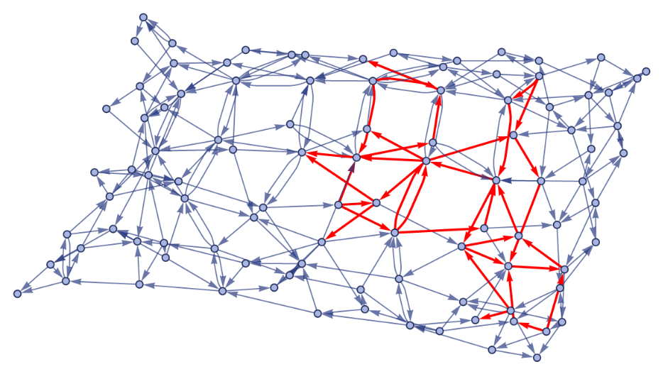
Topological obstructions in a hypergraph that are locally stable under the application of rules are candidates for elementary particles in the Wolfram Model. In this project notebook, we create a hypergraph from a planar, triangular tiling, insert a nonplanar hypergraph or ) as an obstruction, and search for rules in which the obstruction’s effects remained localized using a high-level machine learning-based clustering analysis method. Ultimately, we create an initial framework for generating conditions that exhibit behavior in the Wolfram Model analogous to the motion of an elementary particle in spacetime. There are some promising preliminary results, but much more data needs to be generated in order confirm these results and effectively continue the search for elementary particles. Once a robust framework has been set up for the classification of individual elementary particles, multiple particles should be added to the system to explore analogies to quantum statistics or the dynamics of virtual particles in the quantum foam.
(
K
5
K
3,3
I. Introduction
I. Introduction
A unifying theory of quantum mechanics and general relativity has remained elusive for theoretical physicists who have been especially frustrated by this problem since the mid-20th century when the Standard Model was created to model electromagnetic and nuclear interactions via a quantum field theory. The Wolfram Model provides a unique perspective on the generation of spacetime, one which may provide the discrete features required by quantum mechanics while also adhering to the curvilinear features required by general relativity [1]. In the Wolfram Model, a discrete spacetime mesh is modeled by a hypergraph that evolves under the application of rules like a cellular automaton. In order to connect this model to existing theories in physics, there needs to be an established framework for generating behavior analogous to that of elementary particles moving through spacetime. There are only two structures whose variations cause nonplanarity in graphs: and . We will insert these structures into planar graphs as perturbations and use rules that preserve planarity with the hope that the evolution of this hypergraph will reveal a protected topological obstruction that behaves like a particle (not spontaneously annihilated) as it moves through spacetime. We use a planar, triangular tiling for our spacetime mesh and search for rules that will only make localized changes in this hypergraph. A high-level machine-learning based clustering analysis method will be used to search for a cluster of rules that generate this type of change in the perturbed space’s evolution. The structure of this project notebook is as follows: in section II, we demonstrate how we will create the discrete spacetime mesh. In section III, we show how we will insert as a perturbation the nonplanar graph into the spacetime mesh. In section IV, we detail the methods and tools we will use to determine which rules create particle-like behavior given our initial conditions. In section V, we acquire and analyze the data for and search for rules that generate candidates for elementary particles. In section VI, we similarly acquire and analyze the data for . In section VII, we summarize the results and present suggestions for future work.
K
5
K
3,3
K
5
K
5
K
3,3
II. Creating the discrete spacetime mesh
II. Creating the discrete spacetime mesh
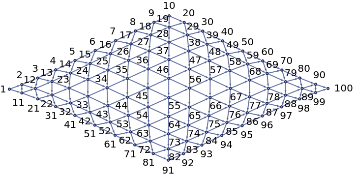
We will begin our search for elementary particle behavior by generating a discrete spacetime mesh. Below, we generate as a demonstration a 10x10 vertex hypergraph comprised of a planar, triangular tiling.
unpertHypergraph=tileTriHGraph[10,10];[unpertHypergraph,VertexLabelsAutomatic,ImageSizeMedium]
Out[]=
The next step is to insert a nonplanar hypergraph as a perturbation which is intended to be analogous to inserting an elementary particle into the discrete spacetime mesh.
III. Inserting K5 into the the spacetime mesh
III. Inserting into the the spacetime mesh
K
5
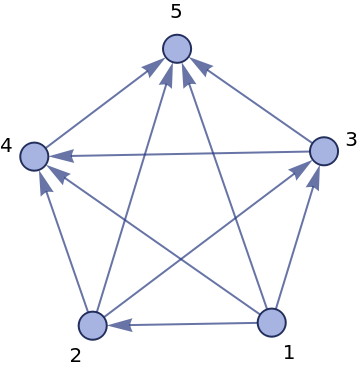
The first nonplanar graph we will insert into our spacetime mesh is , which we can see displayed as a hypergraph below.
K
5
k5={{1,2},{1,3},{1,4},{1,5},{2,3},{2,4},{2,5},{3,4},{3,5},{4,5}};[k5,VertexLabelsAutomatic,ImageSizeSmall]
Out[]=
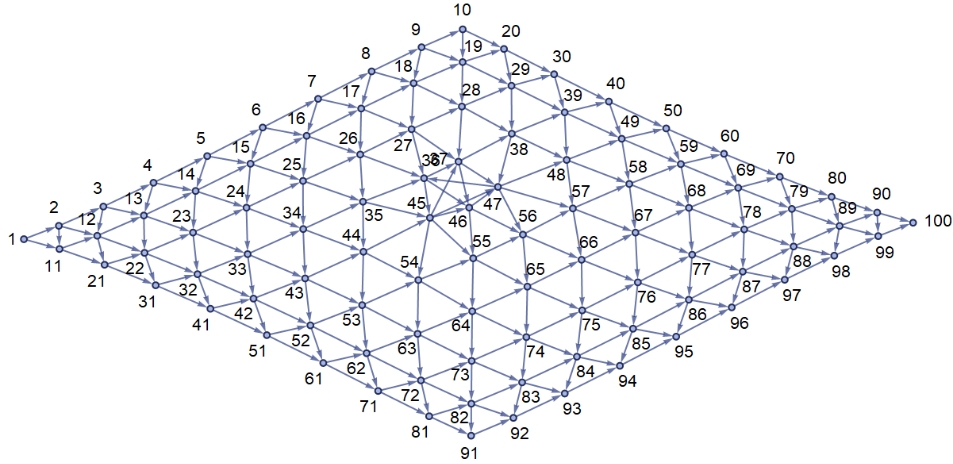
We insert the hypergraph approximately into the center of the spacetime mesh.
K
5
pertHypergraph=pertK5[unpertHypergraph];[pertHypergraph,VertexLabelsAutomatic,ImageSizeLarge]
Out[]=
Now, we need to create the tools to generate the appropriate data to search for elementary particle behavior.
IV. Create the tools to search for rules that generate elementary particle behavior
IV. Create the tools to search for rules that generate elementary particle behavior
We want to find rules that result in localized changes in the evolution of perturbed hypergraphs. In the case of this project, the rules need to have the following specific properties: we want to be able to specify some range of vertices for which we can generate all of the rules that preserve the planarity, vertex number, and edge number of the associated connected graphs. Let us visualize, for example, all of the connected, planar graphs with 4 vertices and 4 edges in randomized directions below.
fourVtx4Edge=dirConnPlanarGraphs[4,4]
Out[]=
,
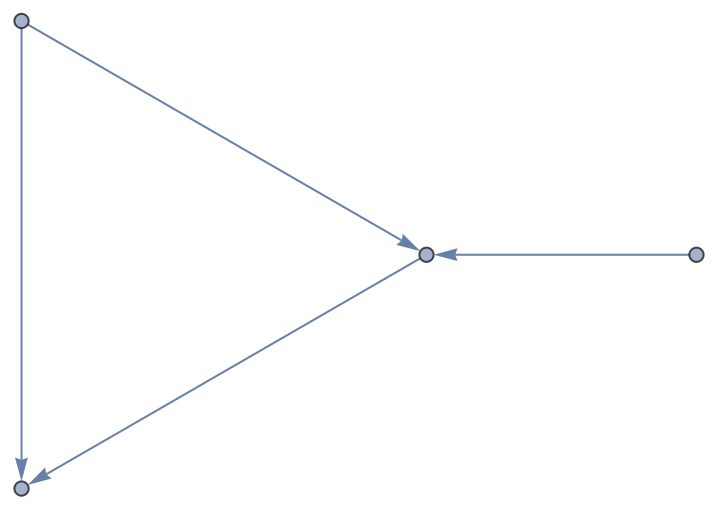

We convert these directed graphs into rules that can be recognized by the appropriate Wolfram Model resource function. We can demonstrate this below for the first directed graph in the list above.
fmtdFourVtx4Edge=fmtDirGraph[fourVtx4Edge[[1]]]
Out[]=
{{1,2},{1,3},{3,2},{4,3}}
We can now turn these formatted directed graphs into rules recognizable by the appropriate Wolfram Model resource function.
fourVtx4EdgeRules=genAllRules[4,4]
Out[]=
{{{{x,y},{x,z},{y,z},{z,w}}{{y,x},{w,x},{z,y},{w,z}}},{{{y,x},{w,x},{z,y},{w,z}}{{x,y},{x,z},{y,z},{z,w}}}}
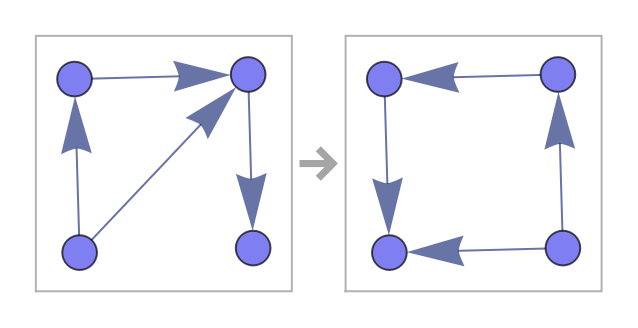
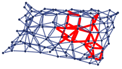
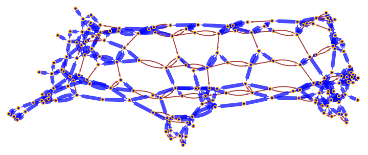
We are interested in collecting the following data: the rule, a plot of the rule (to make it more human-readable), a plot that highlights in red the difference in the evolutions of the perturbed and unperturbed hypergraphs, a plot that highlights in blue the differences in their associated causal graphs (this might give us an analogy to the world line of our particle), and the number of steps of evolution of the unperturbed hypergraph (to see if the rule is associated with a quick termination). Let us see, for example, what this data looks like for the first rule we generated above after 10 steps of the evolution of our hypergraph.
dataDemo=pertGraphData[fourVtx4EdgeRules[[1]],pertHypergraph,unpertHypergraph,10]
Out[]=
{{{x,y},{x,z},{y,z},{z,w}}{{y,x},{w,x},{z,y},{w,z}}},
,
,
,11
We will generate all of the permutations of the rules for any range of vertices and plug them into the appropriate Wolfram Model resource functions. We can see what this looks like for just 4 vertices below.
rulesMat=planarityPrsvngRules[4,4]//MatrixForm
Out[]//MatrixForm=
{{{x,w},{y,w},{w,z}}{{y,x},{z,y},{w,z}}} | |
{{{y,x},{z,y},{w,z}}{{x,w},{y,w},{w,z}}} | |
{{{x,y},{z,x},{y,z},{z,w}}{{y,x},{w,x},{z,y},{z,w}}} | |
{{{y,x},{w,x},{z,y},{z,w}}{{x,y},{z,x},{y,z},{z,w}}} |

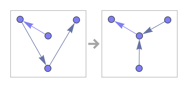
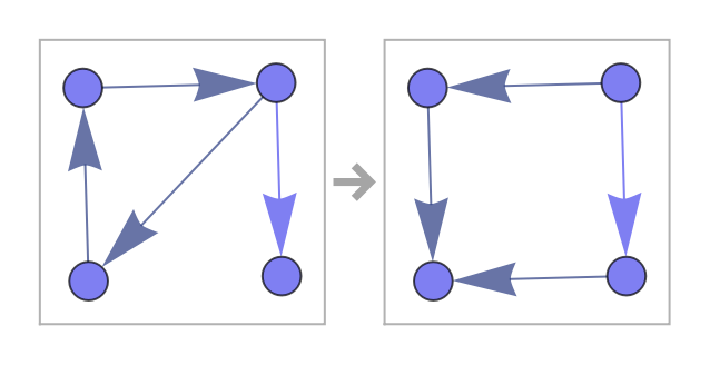
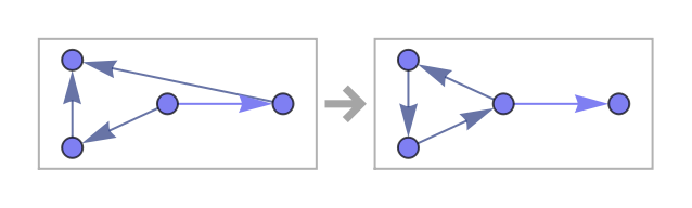
Let us demonstrate the generation of a dataset containing the data for all permutations of rules with 4 vertices for 10 steps of evolution and visualize the first two rows of the data.
We can see that in these two cases, the changes caused by the perturbation have spread out throughout the entire mesh. We are instead looking for more localized changes.
Now, we will use a high-level machine learning based clustering analysis method to see if we can cluster data by its index in the dataset. The results here are not of particular interest since this dataset is relatively small - but this example is meant to demonstrate the process that will be used later on the larger dataset. What we ultimately would like to see is the data split into three clusters - one where the evolution is trivial, one where the changes spread, and one where the changes remain localized.
Now, we will use a high-level machine learning based clustering analysis method to see if we can cluster data by its index in the dataset. The results here are not of particular interest since this dataset is relatively small - but this example is meant to demonstrate the process that will be used later on the larger dataset. What we ultimately would like to see is the data split into three clusters - one where the evolution is trivial, one where the changes spread, and one where the changes remain localized.
Now that we have seen the data acquisition process, let us look for elementary particle behavior in rules that involve more vertices.
The first step to acquiring our data is to generate the spacetime mesh. The mesh here can be made to be rather large but due to time and computational cost constraints we will continue for now with a 10x10 vertex mesh.
Now we acquire the data and save it to a file. In this case, we search from 4 to 5 vertices for up to 10 steps of evolution.
Now let us look for clusters in the dataset.
The clustering analysis method clustered the hypergraphs into 26 groups: 1 cluster with 39 trivial evolutions and 25 separate clusters each containing one hypergraph that has a nontrvial evolution. There was an attempt to force the cluster into the 3 groups mentioned before but not enough data has been generated yet for a clustering analysis method to efficiently work. However, the framework for doing so is in place for future work that will generate larger sets of data. The rules with that generate the most interesting evolutions of our hypergraph can be seen below. The changes are localized, the causal graphs are mostly connected, and they did not terminate quickly. These may be good candidates for elementary particle behavior in the Wolfram Model. Tests on larger sets of data should be run to confirm these preliminary results.
We again start by generating our spacetime mesh.
Now we can collect the evolution data. Again, we will be looking at all permutations of the rules with 4 and 5 vertices for 10 steps of evolution and then saving the file.
Now we want to import the file and find clusters in the dataset.
The clustering analysis method produced a similar result to the last section. There were 20 clusters, one containing 45 trivial solutions and 19 individual clusters which contained each one single nontrivial solution. With more data in future trials the clustering analysis method should be more effective at sorting out the interesting evolutions. The most interesting rules for this perturbation of our hypergraph are shown below.
None of the terminate quickly, they are all fairly localized, and the changes in their causal graphs seem to represent mostly connected world lines. The third rule in this dataset is particularly interesting because of its connected causal graph, but its changes in the hypergraph evolution appear to be slightly more spread out than we might hope to see. With more time and data this rule should be checked in the future for the persistence of this interesting behavior.
Summary and Conclusions
Summary and Conclusions
Keywords
Keywords
◼
Wolfram Model
◼
Topological Obstruction
◼
Machine Learning
◼
Clustering Analysis
Acknowledgement
Acknowledgement
References
References
[1] Wolfram, Stephen. “A Class of Models with the Potential to Represent Fundamental Physics.” Complex Systems 29.2 (2020): 107–536. Crossref. Web.