Introduction
Introduction
Geodesics are fundamental in general relativity. They provide the shortest path between two events and describe the motion of particles in curved spacetime. They also explain the movement of almost all bodies in the Universe due to the rarity of external forces. Although rotating extended bodies do not strictly follow geodesics, their motion can be approximated as geodesic when the spin-curvature interaction is negligible. While studying individual geodesics is crucial in physics, such as understanding the precession of Mercury’s perihelion, examining a congruence of geodesics allows us to address more fundamental questions and explore the nature of horizons in specific spacetimes. For instance, using the Raychaudhuri equation for a congruence of geodesics provides the expansion parameter. This helps us understand that gravity is always attractive, provided the strong energy condition holds throughout all regions of spacetime. Let be an open region in spacetime. A congruence in is a family of curves such that through each point in there passes one and only one curve from this family. In this notebook, we will be interested in congruences of timelike geodesics in a random sprinkling of points in a flat 1+1-dimensional spacetime. This can be enhanced and/or extended to higher-dimensional curved spacetimes.
n
Setting Up the Spacetime
Setting Up the Spacetime
Here, we generate a sprinkling of points in a flat 1+1-dimensional spacetime. This is a discrete two dimensional flat spacetime with events.
n
n
In[]:=
dimensions=2;events=100;SeedRandom[1234];sprinkling=ResourceFunction["FlatSpacetimeSprinkling"][dimensions,events]
Out[]=
SpacetimeSprinkling


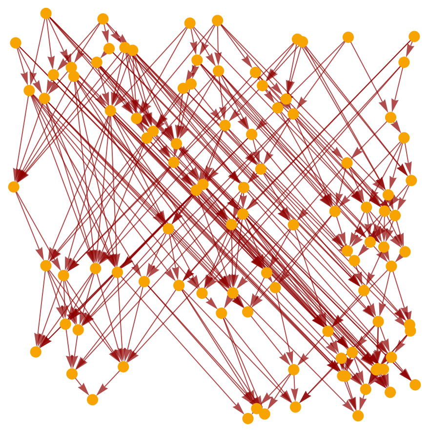
The casual graph associated to the defined events in the spacetime is shown in the following figure.
In[]:=
cg=sprinkling["CausalGraph"]
Out[]=
Geodesics
Geodesics
Maximal means we' re only looking at the longest ones in the scattering, by choosing endpoints that have no ingoing/outgoing vertices
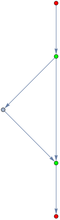
We are only looking at the longest paths in the casual graph. To clarify, let’s assume the following path is part of our causal graph.We are interested in the shortest path between the red points. While the green points are also part of the graph and we could seek the shortest path between them, we notice that they lie on a longer path connecting the red points. Therefore, the following code excludes such paths from our congruence. The idea is to exclude points whose in-degree or out-degree is not zero. The following function, gives us all the possible geodesics between any two pair of separated events.
In[]:=
findGeodesics[cg_Graph]:=Module[{geo=Select[Tuples[{Select[VertexList[cg],VertexInDegree[cg,#]===0&],Select[VertexList[cg],VertexOutDegree[cg,#]===0&]}],GraphDistance[cg,First[#],Last[#]]!=Infinity&]},geo=FindShortestPath[cg,First[#],Last[#]]&/@geo;Graph[DirectedEdge@@@Partition[#,2,1]]&/@geo]
In[]:=
maxgeo=Select[Tuples[{Select[VertexList[cg],VertexInDegree[cg,#]===0&],Select[VertexList[cg],VertexOutDegree[cg,#]===0&]}],GraphDistance[cg,First[#],Last[#]]!=Infinity&];
Now that we have excluded the middle points, we find the shortest path between the events using the following codes:
In[]:=
geopaths=FindShortestPath[cg,First[#],Last[#]]&/@maxgeo;pathedges=Graph[DirectedEdge@@@Partition[#,2,1]]&/@geopaths;
When computing geodesics, we only consider the shortest path between possible endpoints in the sprinkling. Therefore, we might end up excluding vertices that appear in longer paths connecting endpoints.
In[]:=
IsomorphicGraphQ[GraphUnion@@findGeodesics[cg],cg]
Out[]=
False
One can show all such geodesics in the spacetime in the following figure: (Since the following code generates an image, which increases the notebook’s size, I have added a “;” at the end. Remove it if you want to visualize the geodesics.)
In[]:=
HighlightGraph[cg,#,GraphHighlightStyle->"DehighlightHide"]&/@findGeodesics[cg];
Congruence of the Geodesics
Congruence of the Geodesics
Now, we are ready to identify the congruences of the geodesics from the previous section. The following function classifies all non-intersecting geodesics as a congruence.
In[]:=
findCongruences[cg_Graph]:=Module[{geos=findGeodesics[cg],pairwise,cong},pairwise=Association[With[{geo=#},geo->Sort[Select[geos,Intersection[VertexList[#],VertexList[geo]]==={}&]]]&/@geos];cong=Module[{other=pairwise[#]},Append[FixedPoint[If[VertexCount[GraphUnion@@#]<Total[VertexCount/@#],Most[#],#]&,other],#]]&/@Keys[pairwise]]
In[]:=
congruences=findCongruences[cg];
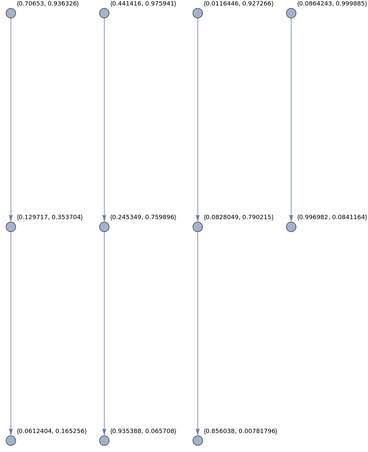
For example, the first congruence is as follows:
In[]:=
Graph[GraphUnion@@congruences[[1]],VertexLabels->Automatic]
Out[]=
It might be interesting, though not necessarily illuminating, to show a specific congruence in the original causal graph. To do so, we should first convert the causal graph to a graph by running the following code.
In[]:=
graph=Graph[EdgeList[sprinkling["CausalGraph"]]]
Out[]=
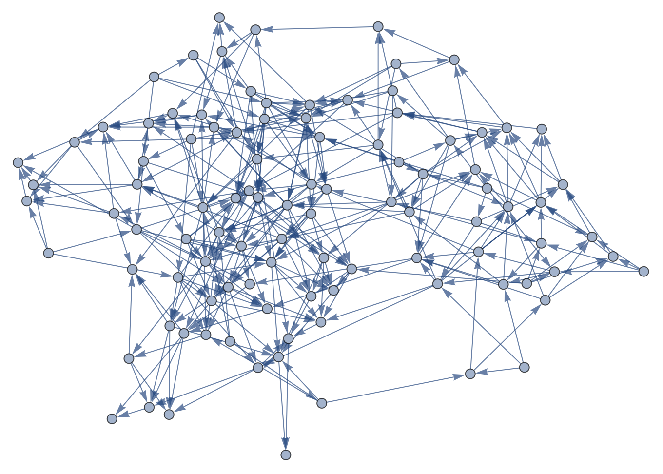
In the following, we show the first congruence in the graph as an example:
Discussion and Future Direction
Discussion and Future Direction
A more interesting case is finding congruences in 4-dimensional curved spacetime. We should note that the ResourceFunction[...Sprinkling] only generates at most 3-dimensional spacetimes. By removing this restriction, we can solve the problem for a more realistic scenario. Additionally, it will be intriguing to explore how one can find geodesic congruences in curved spacetimes with specific metrics, such as Schwarzschild, Kerr, or even dynamical situations like the McVittie black hole.
In this project, we successfully obtained a family of timelike congruences in 1+1 dimensional flat spacetime. Although this spacetime is highly simplified, the lessons learned here can guide us in performing more significant calculations in more realistic scenarios. While solving the geodesic equation in general relativity can be challenging, implementing this method in discrete spaces allows us to find the shortest path between events. However, a potential challenge remains in how to single out specific classes of congruences, such as radial timelike congruences or hypersurface-orthogonal congruences.
For example, the Raychaudhuri equation for a congruence of the timelike geodesics. In four dimensions it reads
Acknowledgment
Acknowledgment
I would like to thank Stephen Wolfram for suggesting this project and Xerxes D. Arsiwalla for his valuable discussions. I extend my deepest gratitude to Mano Namuduri for guiding me through the project with exceptional patience and support.
CITE THIS NOTEBOOK
CITE THIS NOTEBOOK
Geodesic congruence in casual graphs
by Reza Saadati
Wolfram Community, STAFF PICKS, January 16, 2025
https://community.wolfram.com/groups/-/m/t/3357930
by Reza Saadati
Wolfram Community, STAFF PICKS, January 16, 2025
https://community.wolfram.com/groups/-/m/t/3357930