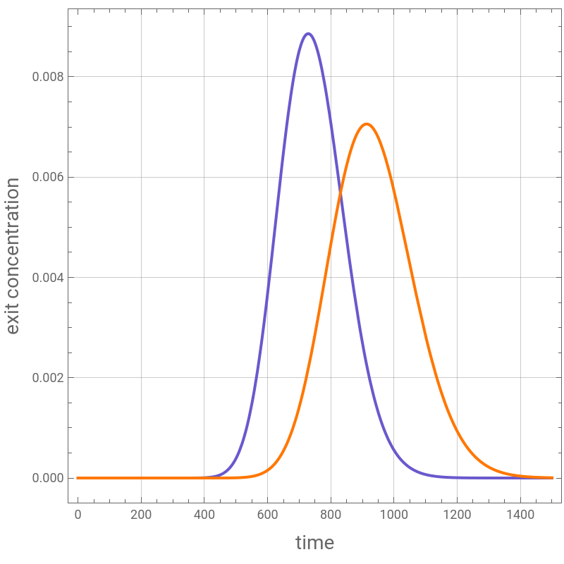
The stagewise (plate) model used here represents a chromatographic column as a cascade of NS ideal equilibrium stages, each behaving as a well - mixed tank in which the mobile and stationary phases are in instantaneous linear equilibrium (q=K C). A rectangular pulse of components A and B (equilibrium constants KA = 0.9 and KB = 1.3) is fed at the column inlet, and the resulting elution profiles at the outlet were obtained by integrating the resulting system of linear ODEs for two values of the stage count, NS = 50 and NS = 500.
Several features of the reconstructed elution peaks are worth highlighting:
• Order of elution and selectivity . Because component A adsorbs less strongly than component B (KA<KB), A spends less time bound to the stationary phase on average and therefore its peak elutes before that of B in both cases. The separation between the two peaks is governed by the difference in the equilibrium constants (the selectivity), not by their absolute values.
• Effect of the number of stages on peak shape . With NS = 50 the two peaks are broad and overlap significantly, producing a “sloppy” separation . Increasing the stage count to NS = 500 produces markedly narrower, taller, and better resolved peaks for the same feed pulse and flow conditions . This mirrors the role of the number of theoretical plates in classical plate theory : more stages (equivalently, a larger number of theoretical plates or a smaller HETP) reduce the effective axial dispersion of the model and sharpen the reconstructed chromatogram, improving resolution between the two elution peaks.
• Peak symmetry . Both peaks remain symmetric (Gaussian-like) in every case, which is a direct consequence of assuming a linear adsorption isotherm . A concentration - independent equilibrium constant guarantees that the governing equations remain linear, so no fronting or tailing appears . In real chromatographic separations, isotherms are often nonlinear (e . g ., Langmuir - type) at higher concentrations, which introduces peak asymmetry — tailing when the isotherm is convex and fronting when it is concave— an effect that this linear model cannot reconstruct.
• Broadening with elution time/dispersion . As anticipated, the more retained species (B) elutes later and its reconstructed peak is broader and shorter than that of the less retained species (A), consistent with the cumulative effect of dispersion (numerical mixing introduced by the finite number of stages) acting over a longer residence time.
• Practical implications . These peaks reproduce, in a simple and computationally cheap way, the well - known trade - off in column design and operation : increasing the number of equilibrium stages (in practice, using a longer column, smaller particles, or otherwise reducing the height equivalent to a theoretical plate, HETP) improves resolution but does not change selectivity, which is set purely by the thermodynamics of adsorption (the equilibrium constants). Achieving a good separation therefore generally requires both sufficient selectivity between species and a sufficiently efficient (high - plate - count) column . Possible extensions of this notebook include : introducing a nonlinear (e . g ., Langmuir) isotherm to reconstruct peak asymmetry and overloading effects; adding explicit mass - transfer resistance between the phases; relating the stage count NS to a physical HETP via the van Deemter equation; and exploring the effect of the feed pulse width and flow rate on resolution and production throughput.
Peak Reconstruction via Moments
Peak Reconstruction via Moments
Rather than plotting peak shape purely from the time-domain solution of the stage-by-stage ODEs, a classical and very economical alternative in chromatography is to characterize (and effectively reconstruct) each elution peak through its statistical moments.
For a concentration profile C(t) at the column outlet, the moments are defined as:
• Zeroth moment (area): total mass eluted.
• First moment (mean retention time): the center of gravity of the peak.
• Second central moment (variance): governs peak width/broadening.
• Third central moment → skewness: measures asymmetry (tailing/fronting).
• Fourth central moment → excess kurtosis: measures peakedness/flatness relative to a Gaussian.
The appeal of this approach is that for a linear plate model these moments can be obtained analytically, directly from the transfer function of the stage cascade (via its Laplace transform or moment-generating function), without ever solving the full time-domain ODE system. However, here we compute the first two moments and use them to plot the Gaussian-like peaks.
Why NS = 500 gives more Gaussian-like peaks than NS = 50
The N-stage equilibrium cascade responding to an impulse (or narrow pulse) is mathematically equivalent to an Erlang (Gamma) distribution with shape parameter N. Its moments have closed forms:
• Skewness decays as 1/. Going from NS = 50 to NS = 500 (a 10× increase) reduces skewness by a factor of 3.16 — e.g., roughly 0.28 at NS = 50 versus about 0.09 at NS = 500. The peak becomes visibly more symmetric.
NS
• Excess kurtosis decays as 1/NS. The same 10× increase in stage count reduces kurtosis by a full factor of 10 — e.g., roughly 0.12 at NS = 50 versus about 0.012 at NS = 500. Kurtosis vanishes even faster than skewness, so the peak rapidly loses its residual peakedness relative to a true Gaussian.
This is a direct manifestation of the Central Limit Theorem: each stage contributes an approximately independent increment to the total residence time, so the outlet concentration profile is (up to normalization) the distribution of a sum of N such increments. As NS grows, that sum converges to a normal distribution, and the rate of convergence is exactly captured by the 1/ and 1/NS decay of skewness and kurtosis.
Practically, this is why the NS = 500 simulation in the notebook produces peaks that look much closer to ideal Gaussians than the “sloppy,” visibly skewed peaks at NS = 50 — it isn’t just that the peaks got narrower, it’s that the higher-order moments (asymmetry and flatness) are being suppressed faster than the width itself shrinks.
NS
Practically, this is why the NS = 500 simulation in the notebook produces peaks that look much closer to ideal Gaussians than the “sloppy,” visibly skewed peaks at NS = 50 — it isn’t just that the peaks got narrower, it’s that the higher-order moments (asymmetry and flatness) are being suppressed faster than the width itself shrinks.
Base case - sloppy separation with NS=50
Equilibrium constants
KA=0.9;KB=1.3;
Total volume
V
tot
50 well-mixed stirred tanks or 50 perfect equilibrium stages
NS=50;
Stage volume
V
stage
V
tot
Volumetric flow rate
L=0.4;
Void fraction
ϵ=0.4;
Column diameter
Dc=4;
Column length
Lbed=25;
In[]:=
eq[i_]:=D[[t],{t,1}]L([t]-[t])ϵ+(1-ϵ)KA;eq2[i_]:=D[[t],{t,1}]L([t]-[t])ϵ+(1-ϵ)KB;eqn=Table[eq[i],{i,1,50}];
CA
i
CA
i-1
CA
i
V
stage
V
stage
CB
i
CB
i-1
CB
i
V
stage
V
stage
In[]:=
initialCond=Table[[0]0,{i,1,50}];sys=Flatten[Join[eqn,initialCond]];Unknown=Table[,{i,1,50}];eqn2=Table[eq2[i],{i,1,50}];initialCond2=Table[[0]0,{i,1,50}];sys2=Flatten[Join[eqn2,initialCond2]];Unkn2=Table[,{i,1,50}];
CA
i
CA
i
CB
i
CB
i
In[]:=
CA
0
CA
init
CA
init
CB
0
CB
init
CB
init
In[]:=
sol1=NDSolve[sys,Unknown,{t,0,5000}];sol2=NDSolve[sys2,Unkn2,{t,0,3000}];
plt2=Plot{Evaluate[[t]]/.sol1,Evaluate[[t]]/.sol2},{t,0,1500},
CA
50
CB
50
Out[]=


Resolution (Rs) separation criterion
Resolution (Rs) separation criterion
Match the upper t-limit used in NDSolve/Plot for this case
tmax=2000;
In[]:=
cA[t_]:=Evaluate[[t]]/.sol1[[1]]cB[t_]:=Evaluate[[t]]/.sol2[[1]]
CA
50
CB
50
Zeroth moment:area under each peak
areaA=NIntegrate[cA[t],{t,0,tmax}];areaB=NIntegrate[cB[t],{t,0,tmax}];
First moment:retention time (mean elution time)
tRA=NIntegrate[t*cA[t],{t,0,tmax}]/areaA;tRB=NIntegrate[t*cB[t],{t,0,tmax}]/areaB;
Second central moment: variance->sigma
varA=NIntegrate[(t-tRA)^2*cA[t],{t,0,tmax}]/areaA;varB=NIntegrate[(t-tRB)^2*cB[t],{t,0,tmax}]/areaB;sigmaA=Sqrt[varA];sigmaB=Sqrt[varB];
Third central moment: skewness
sA=NIntegrate[(t-tRA)^3*cA[t],{t,0,tmax}]/sigmaA^3/areaA;sB=NIntegrate[(t-tRB)^3*cB[t],{t,0,tmax}]/sigmaB^3/areaB;
In[]:=
{sA,sB}
Out[]=
{0.282538,0.282593}
In[]:=
2Sqrt[50.](*checkskewnessshouldbe2
NS
*)Out[]=
0.282843
Fourth central moment: kurtosis
kA=Quiet@NIntegrate[(t-tRA)^4*cA[t],{t,0,tmax}]/areaA;kB=Quiet@NIntegrate[(t-tRB)^4*cB[t],{t,0,tmax}]/areaB;
Normalized (dimensionless) kurtosis and excess kurtosis
kurtA=kA/sigmaA^4;kurtB=kB/sigmaB^4;excessKurtA=kurtA-3;excessKurtB=kurtB-3;
In[]:=
{kurtA,kurtB}(*foraGaussianprofilethiskurtosisshouldbeequalto3*)
Out[]=
{3.11964,3.11951}
Baseline peak width,Gaussian approx: w = 4*sigma
wA=4*sigmaA;wB=4*sigmaB;
Resolution
Rs=2*(tRB-tRA)/(wA+wB);Print["Retention time A = ",NumberForm[tRA,5]];Print["Retention time B = ",NumberForm[tRB,5]];Print["Peak width A (4σ) = ",NumberForm[wA,5]];Print["Peak width B (4σ) = ",NumberForm[wB,5]];Print["Resolution Rs = ",NumberForm[Rs,4]];
Case study 2 - separation with NS=500
Case study 2 - separation with NS=500
Equilibrium constants
Total volume
500 well-mixed stirred tanks or 500 perfect equilibrium stages
Stage volume
Volumetric flow rate
Void fraction
Column diameter
Column length
Resolution (Rs) separation criterion
Match the upper t-limit used in NDSolve/Plot for this case*
Zeroth moment:area under each peak
First moment:retention time (mean elution time)
Second central moment: variance->sigma
Third central moment: skewness
Fourth central moment: kurtosis
Normalized (dimensionless) kurtosis and excess kurtosis
For a Gaussian profile this kurtosis should be equal to 3
Baseline peak width,Gaussian approx:w=4*sigma
Resolution
Since NS is large (NS=500) perfect overlap between computed and reconstructed (Gaussian-like) peaks is observed
Reference
Reference
[1] J. Ingham, I. J. Dunn, E. Heinzle, and J. E. Prenosil, “CHROMPLATE - Stagewise Model for Chromatography Columns,” Chemical Engineering Dynamics, 2nd ed., Weinheim, Germany: Wiley-VCH, 500 pp. 541–545.
CITE THIS NOTEBOOK
CITE THIS NOTEBOOK
Chromatographic peak reconstruction via stagewise plate model with linear adsorption
by Housam Binous
Wolfram Community, STAFF PICKS, August 11, 2026
https://community.wolfram.com/groups/-/m/t/3779221
by Housam Binous
Wolfram Community, STAFF PICKS, August 11, 2026
https://community.wolfram.com/groups/-/m/t/3779221