Introduction
Introduction
Global warming is the current rise of the average temperature on Earth as a result of the changing climate. Mostly due to human activity, there has been a recent increase in surface temperatures and sea levels, more severe and frequent natural disasters, and more. These changes to our climate have not only impacted the human population, but also other animal species that cannot adapt to this new environment. Two of the biggest contributors to climate change is accelerating carbon emissions and deforestation, both caused by humans. There have been some studies showing the correlation between land use and greenhouse gas emissions. This project, which I made at the Wolfram Summer Camp with the help of mentors, aims to provide evidence for the relationship between land usage and carbon monoxide emissions. I hope the results of this project can be used to further educated people and present the urgency for change.
The goal of this project was to display the correlation between land usage and carbon monoxide levels in a country. Land cover type and carbon monoxide emissions data were extracted and interpreted from the NASA Earthdata repository to create visuals, either in the form of maps or graphs, of user-specified countries. The data derived from the maps were then used to create plots that show change over time when comparing the data from two countries or within one country.
The goal of this project was to display the correlation between land usage and carbon monoxide levels in a country. Land cover type and carbon monoxide emissions data were extracted and interpreted from the NASA Earthdata repository to create visuals, either in the form of maps or graphs, of user-specified countries. The data derived from the maps were then used to create plots that show change over time when comparing the data from two countries or within one country.
Extracting the Data
Extracting the Data
The imported NASA Earthdata contained information for world land usage from 2001 to present and carbon monoxide levels from 1980 to present. Since the online repository is formatted in XML, the data had to be modified. The code to do this was created by Christopher Wolfram.
Imports the data from the NASA Earthdata repository:
rawXML=Import["https://gibs.earthdata.nasa.gov/wmts/epsg3857/best/1.0.0/WMTSCapabilities.xml"];
Accesses the information within the many layers in the NASA Earthdata:
layers=Module[{rawLayers,layers},rawLayers=Cases[rawXML[[2,3,4,3]],XMLElement["Layer",_,_]][[All,3]];Association[Function[xml,Module[{id},id=FirstCase[xml,XMLElement[{"http://www.opengis.net/ows/1.1","Identifier"},_,{identifier_}]identifier];id<|"Title"FirstCase[xml,XMLElement[{"http://www.opengis.net/ows/1.1","Title"},_,{t_}]t],"TileMatrixSet"FirstCase[xml,XMLElement["TileMatrixSetLink",{},{XMLElement["TileMatrixSet",{},{tms_}]}]tms],"Template"StringTemplate@StringReplace[FirstCase[xml,XMLElement["ResourceURL",{OrderlessPatternSequence[___,"template"t_]},_]t],{"{Time}""<*DateString[#Time,{\"Year\",\"-\",\"Month\",\"-\",\"Day\"}]*>","{"~~Shortest[name__]~~"}""`"<>name<>"`"}],"DateRange"FirstCase[xml,XMLElement["Dimension",{},{OrderlessPatternSequence[___,XMLElement[{"http://www.opengis.net/ows/1.1","Identifier"},{},{"Time"}],XMLElement["Value",{},{v_}]]}]DateObject/@StringSplit[v,"/"][[;;2]]],"DateDefault"FirstCase[xml,XMLElement["Dimension",{},{OrderlessPatternSequence[___,XMLElement[{"http://www.opengis.net/ows/1.1","Identifier"},{},{"Time"}],XMLElement["Default",{},{d_}]]}]DateObject[d]]|>]]/@rawLayers]];
Creates an Association[] between the levels within the imported data and {1, level number}:
tileMatrixZoomLevels=<|"GoogleMapsCompatible_Level6"{1,6},"GoogleMapsCompatible_Level7"{1,7},"GoogleMapsCompatible_Level8"{1,8},"GoogleMapsCompatible_Level9"{1,9},"GoogleMapsCompatible_Level12"{1,12},"GoogleMapsCompatible_Level13"{1,13}|>;
Withdraws data from the NASA server which can then be used within GeoServer:
layerGeoServer[layer_,time_]/;KeyExistsQ[layers,layer]:={layers[layer]["Template"][<|"Time"time,"TileMatrixSet"layers[layer]["TileMatrixSet"],"TileMatrix""`1`","TileRow""`3`","TileCol""`2`"|>],"ZoomRange"tileMatrixZoomLevels[layers[layer]["TileMatrixSet"]]}layerGeoServer[layer_]:=layerGeoServer[layer,layers[layer]["DateDefault"]]layerGeoServer[]:=layers
Forming an Image
Forming an Image
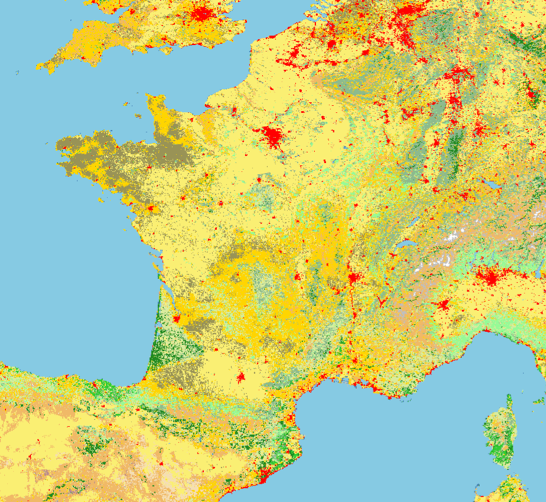
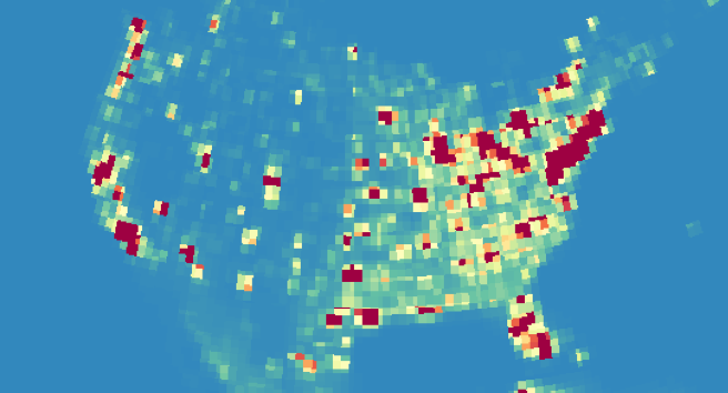
The data from the NASA repository was turned into GeoImage[]s with the GeoServer being provided by layerGeoServer[].The constructed images displayed the region of the specified country along with its data is shown from 2001 to 2017. When entering the specified country, the user must input an Entity[].
Produces land cover type images of France in 2001:
landIMG=GeoImageGeoRange,GeoServerlayerGeoServer["MODIS_Combined_L3_IGBP_Land_Cover_Type_Annual",DateObject[{2001,1}]],GeoProjection"Orthographic"
Out[]=
Constructs carbon monoxide emission images of the United States in 2001:
carbonIMG=GeoImageGeoRange,GeoServerlayerGeoServer["MERRA2_Carbon_Monoxide_Emission_Monthly",DateObject[{2001,1}]],GeoProjection"Orthographic"
Out[]=
Isolating One Country
Isolating One Country
As a result of using GeoImage[] to generate the maps, the image of the country was not isolated.
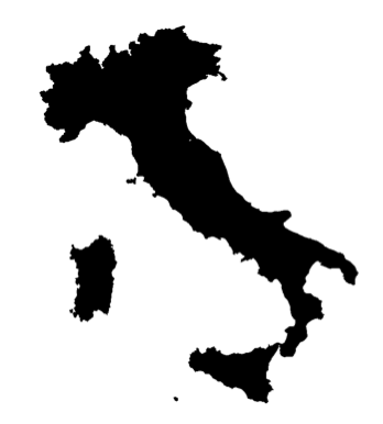
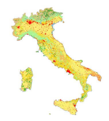
In order to accomplish isolating the country, a mask of the user-specified country was created and applied to the GeoImage. Since the image colors correspond to land type or carbon monoxide levels, the data for the inputted country can be extracted by counting the amount of pixels per color. To fit the mask onto the original image, the dimensions of the mask was changed to the same size as the original. This method was used for both land cover type and carbon emission images.
In order to accomplish isolating the country, a mask of the user-specified country was created and applied to the GeoImage. Since the image colors correspond to land type or carbon monoxide levels, the data for the inputted country can be extracted by counting the amount of pixels per color. To fit the mask onto the original image, the dimensions of the mask was changed to the same size as the original. This method was used for both land cover type and carbon emission images.
Constructs an image of the specified country (Italy), which is then turned into a mask.
carbonORLandMask=ImageResizeColorNegateBinarizeImageGeoGraphicsGeoStyling[None],EdgeForm[Blue],FaceForm[Blue],Polygon,GeoBackgroundNone,GeoProjection"Orthographic",ImageDimensions[carbonOrLandIMG]
Out[]=
Produces the masked image of Italy by applying the mask to the original image:
oneCountryImage=BrightnessEqualize[ImageApply[1-#&,carbonOrLandIMG,MaskingcarbonOrLandMask],1]
Out[]=
Recoloring the Land Cover Type Images
Recoloring the Land Cover Type Images
When the images with land cover data were imported into Mathematica, the colors shifted slightly. These colors needed to match with the ones from the original legend, which were generated from the NASA data. To fix this problem, all the pixels from the masked image were changed using ColorReplace[], where the masked image's colors were replaced with the closest color based on the NASA legend. The pixel colors were changed based on their respective land types, grouping land types together for further analysis.
Generates a recolored land cover type image of Spain in 2001:
Using the Data to Create Images
Using the Data to Create Images
Land Cover Type
Land Cover Type
To create maps that would allow for the analysis of the NASA data, a new image was created that combined the recolored image, a legend, and the percentage of the amount of each land type group for that country. Most of the code used in anyCountryLand[] was taken from previous variables.
Note: all variables below will not generate proper output.
Note: all variables below will not generate proper output.
Creates an association between the amount of pixels and its respective color
Yields the colored image along with a color legend and the percentages of each land cover type:
Develops an image that displays a map, legend, and percentages based on the land cover type data in the United States in 2001:
The anyCountryLand[] function was then used to construct a ListAnimate[] that presented the same data for multiple years. The function allows the user to see data from 2001, 2010, and 2017. These dates were chosen to demonstrate change over time while accounting for many years taking a longer time to run.
Constructs an interactive animation of the land cover type of the United States during the years 2001, 2009, and 2017:
Monthly Carbon Monoxide Emissions
Monthly Carbon Monoxide Emissions
The images created for the carbon monoxide emissions are extremely similar to the ones created for the land cover type data. Using a related strategy for producing the anyCountryLand[] function, the anyCountryCarbon[] function uses the GeoImage, mask, and masked image. While the images with land type data needed to be recolored, the carbon images were not for this function because a Count[] of the pixels was not taken yet. Using carbon data from the NASA site, a legend was created that corresponded the pixel colors to a specific value measured in kg/m^2/s.
Note: all variables below will not generate proper output.
Note: all variables below will not generate proper output.
Constructs a number to color association that is used as a legend:
Rearranges above output into a new association (color to number):
Produces a gradient legend using the input above to create labels:
Produces expected outputted image with a legend:
Yields an image of Turkey with colors that correspond to the amount of carbon monoxide produced across the country during 2007:
The anyCountryCarbon[] function was then used to produce another function similar to the anyCountryLandLA[] function. However, instead of showing land cover types and their percentages, it shows a map of carbon monoxide levels over the same years (2001, 2009, and 2017).
Generates an interactive list animation of carbon monoxide emissions in Turkey during the years 2001, 2009, and 2017:
Comparing Data Through Graphs
Comparing Data Through Graphs
To investigate the correlation between land coverage type and carbon monoxide emissions, plots of the two data sets were produced.
Land Type Cover Values
Land Type Cover Values
To extract the data from the land cover type images, a similar process as anyCountryLand[] was used to create numsLand[]. Using the recolored image, the pixel values were grouped together by color which corresponded to a land type. numsLand[] takes in a specified country, year, and land type(s). The generated values are created by counting the number of pixels from a user-specified land cover type (item) and extracted from cAmounts.
However, after counting the amount of pixels per land type in the image, the colors shifted again. To solve this problem, FindMatchingColor[] was used to find the closest color in the cAmounts association to the colors in the masked image. The named colors from the masked image are called based on the user's input into item_ and is combined with the string "Color".
For item_, a list of land cover types, with all lower case letters, must be entered (i.e. {"forest","crop"}). The user can choose from any of the items: forest, shrub, crop, savanna, urban, and grassland. While the function itself does not produce percentage values, PercentForm[] can be mapped across the output to display these values.
Note: all of the code below besides numsLand[] will not generate proper output.
However, after counting the amount of pixels per land type in the image, the colors shifted again. To solve this problem, FindMatchingColor[] was used to find the closest color in the cAmounts association to the colors in the masked image. The named colors from the masked image are called based on the user's input into item_ and is combined with the string "Color".
For item_, a list of land cover types, with all lower case letters, must be entered (i.e. {"forest","crop"}). The user can choose from any of the items: forest, shrub, crop, savanna, urban, and grassland. While the function itself does not produce percentage values, PercentForm[] can be mapped across the output to display these values.
Note: all of the code below besides numsLand[] will not generate proper output.
Finds the nearest color in the cAmounts association to the colors in the masked image and divides by the total amount of colored pixels:
Generates the percentages of the land cover types: savannas, forests, and crops in Brazil during 2014:
Carbon Monoxide Emission Values
Carbon Monoxide Emission Values
Similar to numsLand[], the numsCarb[] function used some of the same code from anyCountryCarbon[]. However, this function generates the average of carbon monoxide emissions for a specific year and country. Besides taking an average of the carbon monoxide emissions by correlating pixel color with emission amounts, the process is the same as numsLand[]. Also, as seen in numsLand[], the pixel colors changed when counted.
Note: all of the code below besides numsCarb[] will not generate proper output.
Note: all of the code below besides numsCarb[] will not generate proper output.
Creates an association between the amount of pixels and its respective color:
Finds the closest color in cCounts, to the original legend list:
Turns the values in colorsCarbon into numbers:
Generates the average carbon emissions for specified year:
Yields the average of carbon monoxide levels of China in 2009 :
Comparison Graphs For One Country
Comparison Graphs For One Country
In order to compare the numbers generated by numsLand[] and numsCarb[], plots[] was created to display land cover types and carbon emissions for one country over the years 2001, 2005, 2009, 2013, and 2017. plots[] utilizes the functions numsLand[] and numsCarb[] to yield two separate, yet related graphs. Since numsLand[] generates a list of values, unlike numsCarb[], Map[] was used to reformat the list. Then, both carbon emissions and land type were plotted and placed next to each other for straightforward comparison and relationship analysis.
Note: all of the code below besides plot[] will not generate proper output.
Note: all of the code below besides plot[] will not generate proper output.
Produces a list of {year, {values}} using numsLand[]:
Generates a list of {year, {values}} using numsCarb[] :
Constructs a plot that shows land cover type changes over time:
Yields a plot that displays carbon monoxide levels from 2001 to 2017:
Constructs two plots: one shows the United States land cover types: crops, shrubs, and urban areas,
and the second displays their carbon monoxide levels from 2001 to 2017:
and the second displays their carbon monoxide levels from 2001 to 2017:
Conclusion
Conclusion
Results
Results
Although there are no clear correlations between land cover type and carbon monoxide emissions over the years 2001 to 2017, if there was more data on land cover type and a longer time frame for the Wolfram Summer Camp we could investigate further. Unfortunately, NASA's Earthdata only goes back to 2001. Also, another factor could be the small amount of years used to produce the plots and GeoImages. While this project is inconclusive, it still displays interesting information about land type and carbon emissions. I hope someone, or myself, will expand on this project in the future and reach a conclusion.
Further Extensions
Further Extensions
If given more time to complete this project, I would make the code more elegant. Currently, most of the code is quite complicated and takes a while to run because most functions require taking pixels from an image. For example, generating the country list animations is intricate and relies on the anyCountryLand[] or anyCountryCarbon[] function to construct the images. This process is inconvenient for the user since generating the output is slow and one can only see the change over only a few years. It would be interesting to analyze the data over more years to more accurately study the changing data values. Furthermore, most of the images or graphs produced rely on previous inputs which further decreases the speed of the code. Another extension to this project would be to create a function that constructs a graph with the land cover type and carbon emission data of two countries to further investigate the relationship between land usage and carbon monoxide levels.