The Collatz conjecture, or 3n+1 problem, is an unsolved mathematics problem infamous for its ease of explanation yet remarkable difficulty in solvability. The classical Collatz function seems to exhibit a downward bias, meaning sequences tend to decrease over time. This project explores generalized Collatz functions to find “statistically balanced” variants that are equally likely to increase or decrease values, making them theoretically the hardest to prove. By searching functions with zero or near-zero bias across different modular spaces (mod-3 through mod-8), developing bias estimation methods based on coefficient products, and doing statistical analysis, we identify perfectly balanced variants and provide new tools for exploring discrete dynamical systems beyond the classical conjecture.
1: Exploring General Forms of Collatz
1: Exploring General Forms of Collatz
1.1: Overview of the Collatz Problem
1.1: Overview of the Collatz Problem
The Collatz conjecture, also known as the 3n+1 problem, is an unsolved problem in mathematics concerning the behavior of sequences defined by a simple iterative process. Given any positive integer n, the conjecture states that repeated application of the following function will eventually reach the value 1:
F(n)
1 2 | if n≡0 (mod2) |
3n+1 2 | if n≢0 (mod2) and mn≡r(mod2) for r∈R |
Or as a Mathematica function:
In[]:=
f[n_]:=If[EvenQ[n],n/2,3*n+1]
The conjecture asserts that for any initial positive integer, the sequence generated by iteratively applying this function will always eventually reach 1, after which it enters the cycle 1 → 4 → 2 → 1.
Given an initial value, a sequence of numbers can be generated that eventually converges.
In[]:=
NestList[f,11,20]
Out[]=
{11,34,17,52,26,13,40,20,10,5,16,8,4,2,1,4,2,1,4,2,1}
To simplify the number of steps, we can divide (3n+1) by 2. Given this executes when n is odd and upon execution of (3n+1), n becomes even, thus the consecutive step would be the division by n/2. This serves as our basis of the generalizations.
In[]:=
g[n_]:=If[EvenQ[n],n/2,(3*n+1)/2]
An example for using g to generate the Collatz sequence with initial value 11:
In[]:=
NestList[g,11,20]
Out[]=
{11,17,26,13,20,10,5,8,4,2,1,2,1,2,1,2,1,2,1,2,1}
1.2: Generalizations of the Collatz Problem
1.2: Generalizations of the Collatz Problem
There is a few ways to generalize the Collatz Function to other parameters. One such way is through FRACTRAN, created by John Conway. Using the definition from Russel Martinez’s “Exploring generalized Collatz functions”,
In[]:=
collatzList={165/14,11/63,38/21,13/7,34/325,1/13,184/95,1/19,7/11,13/17,19/23,1575/4};Log2@ResourceFunction["Fractran"][collatzList,2^11,MaxResults->25,SelectionCriterion->IntegerQ@*Log2]
Out[]=
{11,34,17,52,26,13,40,20,10,5,16,8,4,2,1}
However, this method complicates the parameters of higher mod numbers and it’s abstract nature made exploring more generalized space difficult. Fortunately, Lagarias’s “The 3x + 1 Problem and its Generalizations” proposed another more direct generalization which will serve as the foundational basis of the exploration of general Collatz.
Itreferstoaclassoffunctionsthatareperiodicallylinearandinvolvemodulararithmeticoperations.
UU(m,d,R)
The function is defined based on the modular condition of with respect to :
U(n)
n
d
U(n)
n d | if n≡0 (mod) |
mn-r d | if n≢0 (mod) and mn≡r(mod) for r∈R |
Keep in mind that for higher there will be more terms that . Therefore the parameter-space increases as increases.
d
n≢0 (mod)
d
This definition allows for the exploration of more generalized behavior in integer sequences by adjusting the parameters , , and . Here it is defined as a Mathematica formula:
m
d
R
In[]:=
collatzGeneral2[coeffs:{{_Integer,_Integer}..},d_Integer,x_Integer]:=With[{m=Length[coeffs]},(coeffs[[Mod[x,m]+1]].{x,1})/d]
Where Coeffs takes in an infinite list of parameters. For example, {{a,b},{c,f}} corresponds to
U(n)
an-b d | if n≡0 (mod) |
cn-f d | if n≢0 (mod) and mn≡r(mod) for r∈R |
Basically the first integer of {a,b} is the coefficient and the second is an additive constant.
Here is an example of collatzGeneral2 recreating the original Collatz function with parameters {{1, 0}, {3, 1}}:
Out[]=
{11,17,26,13,20,10,5,8,4,2,1,2,1,2,1,2,1,2,1,2,1}
In a general parameter space in an given mod number, there exists certain initial conditions that causes a sequence to create non-integer values. To limit the scope of this project, only positive integers will be considered. Therefore, an version of collatzGeneral2 with error handling is created, as shown below:
collatzGeneral3[coeffs_,d_,x_]:=With[{m=Length[coeffs]},Module[{result},(*Validation:ensurecoefficientsanddivisorarevalid*)If[Not[And@@(IntegerQ/@Flatten[coeffs])&&IntegerQ[d]&&d>0&&IntegerQ[x]&&x>0],Return[$Failed]];(*Calculatenextvalue*)result=(coeffs[[Mod[x,m]+1]].{x,1})/d;(*Returnresultonlyifit’sapositiveinteger*)If[IntegerQ[result]&&result>0,result,$Failed]]];
From now on, collatzGeneral3 will be assumed to be the default generalization of a given parameter space.
2: Properties of Selected Divergent Functions
2: Properties of Selected Divergent Functions
2.1 Introduction to the mod-3 Space
2.1 Introduction to the mod-3 Space
The classical Collatz conjecture operates within a mod-2 framework, where each integer is evaluated as either even or odd. This binary approach informs the sequence’s progression by applying different transformations based on the integer’s parity. However, when we extend the problem into a mod-3 space, we introduce an additional layer of complexity. In this space, each integer is classified into one of three categories based on its remainder when divided by 3: , , and .
n≡0 (mod3)
n≡1 (mod3)
n≡2 (mod3)
Similarities and Differences to the Original Collatz Problem
Similarities and Differences to the Original Collatz Problem
While the original Collatz function only requires a mod-2 decision (even or odd), the generalized function in mod-3 space requires handling three distinct cases. This adds a layer of complexity, as the rules for transformation can vary more significantly between cases.
Also In the mod-3 space, different transformation rules can be applied based on the remainder. This allows for more intricate behaviors and potentially more complex sequences, as the transformation is not limited to simply dividing by 2 or applying the 3n+1 rule.
2.2 Exploring a Specific Variation
2.2 Exploring a Specific Variation
In Stephen Wolfram’s writing “After 100 Years, Can We Finally Crack Post's Problem of Tag? A Story of Computational Irreducibility, and More”, the “title” of an “most unbiased” system was conceived to the mod-3 space system {4 n + 2, 7 n + 1}. Plugging it into our general Collatz function,
In[]:=
NestList[collatzGeneral3[{{1,0},{4,2},{7,1}},3,#]&,11,20]
Out[]=
{11,26,61,82,110,257,600,200,467,1090,1454,3393,1131,377,880,1174,1566,522,174,58,78}
We can generate a sample with initial condition 11.
To further study the behavior of the function, we test a random sample of a wide range of values and then take the logarithmic average of a given percentile of the range of initial values. We end up with the following graph:
Out[]=
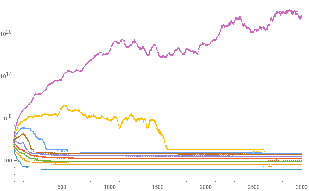


Logarithmic average of sequences’ values along steps. Each colored-line represents a group of sequences partitioned by initial values. For instance, 0.1 represents the bottom 10% of the initial values from 100 to 100000.
Plotted for 3000 steps. The top 10% seemingly diverges while the rest converges within the 3000 step window. Zooming in specifically on the 0.85-1 range and running for more steps, we get this:
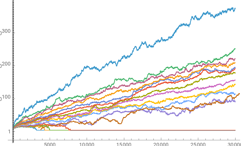


Logarithmic average of sequences’ values along steps. Each colored-line represents a group of sequences partitioned by initial values. For instance, 0.85 represents the bottom 85% of the initial values from 100 to 100000.
These higher range of values seemingly diverges infinitely. It makes sense, as the average bias of a given mod 3 general Collatz is
In[]:=
clgb[a_,b_]:=Log2[(a*b)/27];
where a and b denotes the coefficients of the Collatz function, 4 and 7. The resulting value is:
Out[]=
0.0524674
This means that theoretically, the function have a slight divergent tendency. But why specifically for the larger values? Does the smaller values also diverge?
In this case, 469 serves as a interesting initial condition. It is a relatively small value that resides in the lower 10% range, a majority converging group, but it diverges infinitely.
Out[]=
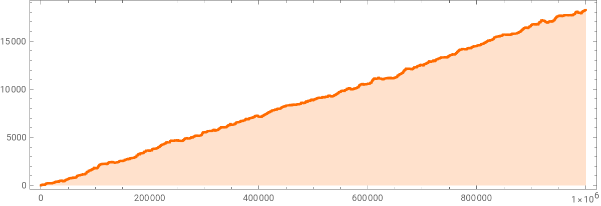
◼
From experimentation, 487, 626, 650 also diverges while being under the 1000 range. The relationship between these numbers were unclear initially however.
Observe the sequence of numbers plotted below using initial condition 469:
It seems that all of the initial conditions that diverges are steps within the 469 sequence, which is an unsurprising discovery. However, this now means that all values that converges onto this infinite sequence of numbers will also diverge. Given the variant is in mod 3 space, there are three ways of reaching any given values. Theoretically, each existing number in the 469 sequence has up to two other branches. Thus it creates a infinitely large space of parameters that will all diverge.
2.3 The Divergence Space
2.3 The Divergence Space
In order to identify which values would converge onto the sequence, a reverse calculation can be performed using the three conditions:
For example, to find which values converge to 469 from the first {1,0} parameter ((n+0)/3), we run:
We call this (infinite) set of values the divergence space of the initial condition 469.
To visualize this space better, we can create an infinitely expanding map of divergent values.
A map of divergent values within the given function. The red line represents the initial strand of divergent values, starting from 469. The grey branches represents other values that converges onto this initial strand.
This creates a series of patterns that looks like tree branches or other organic structures.
Now we aim to answer the question of how many (or how frequently) initial conditions actually merge into the divergence space. In the graph below we show the percentage of divergent initials for each of our percentile sets:
Now we aim to answer the question of how many (or how frequently) initial conditions actually merge into the divergence space. In the graph below we show the percentage of divergent initials for each of our percentile sets:
This graph measure the ratio of divergence values within a specific percentile of initial values.
Further diving into the divergence space, one can see that it is empirically true that divergence is more common among higher values.
We also consider computing the average of values produced by a sequence (running 3000 steps). The general idea is that by the average we have some simple metric that indicates how much the sequence grows (even diverging) or gets stuck in cycles or lower values (likely converging)
The graph belows shows these averages for each initial condition from 1 to 1000.
The graph belows shows these averages for each initial condition from 1 to 1000.
Log Plot of the average of a range (1 to 1000) of initial values, running for 3000 steps.
Also interesting to note is that formation of ‘tiers’. While most averages to the two most common values, some convergent ones managed to reach a very high average as well.
Although the bias prediction - the likely hood of convergence or divergence - states that this specific function has a slight divergence, the behavior of the higher initial values is very different from lower ones. It seems that the low bias values is only attained through the balance of divergent and convergent values within a give window.
2.4 Digits Representation on Specific Collatz Variant
2.4 Digits Representation on Specific Collatz Variant
In addition to the analysis of functional behavior, I also tried to encode the sequence in different numbering system to find the patterns within Collatz. Starting with the original Collatz function, one can encode it’s value in base 2, creating a plot similar to Cellular Automata. This was done with initial values 2^100 + 2^70, which placed two pixels in exact locations on the grid
Collatz Function plotted in Base 2 for 2^100 + 2^70
Here is the same function, but using initial values 2^100+2^70+1 encoding in base 2 as well
Collatz Function plotted in Base 2 for 2^100 + 2^70 + 1
Interestingly, triangular patterns form within the plot. Plotting it in base 3 reveals other forms of repeating triangles.
Collatz Function plotted in Base 3 for 2^100 + 2^70 + 1
And also the two giant white triangles
Here is it plotted in base 6. Notice how the triangular patterns disappear.
Collatz Function plotted in Base 6 for 6^100 + 6^70 + 1
Plotting the specific Collatz variant sequence {{1, 0}, {4, 2}, {7, 1}} results in the following:
Specific Collatz Function {{1, 0}, {4, 2}, {7, 1}} plotted in Base 3 for 2^100 + 2^70 + 1
Let’s try setting the initial cells to specific ones on the grid
Specific Collatz Function {{1, 0}, {4, 2}, {7, 1}} plotted in Base 3 for 3^100 + 3^70 + 1
plotted in binary
Specific Collatz Function {{1, 0}, {4, 2}, {7, 1}} plotted in Base 2
Triangular patterns never existed on this specific function
Specific Collatz Function {{1, 0}, {4, 2}, {7, 1}} plotted in Base 6
Given similar results and structure, one can conclude that there is no real difference between base 2, base 6, or base 3 digit representation. There also isn’t really a coherent repeating pattern like the original Collatz function for this specific varment of Collatz.
We also have tested another convergent form within the mod-3 space to investigate wether the lack of patterns is an effect specific of divergent functions.
Using the bias function mentioned earlier, we found that {{1,0},{4,2},{1,1}} parameters leads to a convergent function in mod-3 space.
Here is the plot in base 6.
Specific Collatz Function {{1,0},{4,2},{1,1}} plotted in Base 6
This lack of triangular pattern seems to be universal across the mod - 3 space, although more testing is needed to determine such a conclusion.
3: Parameter Validation and Collatz Bias
3: Parameter Validation and Collatz Bias
3.1 Defining Bias
3.1 Defining Bias
A natural transformation of the bias function to the mod - 2 space is:
Specifically, for the 3n + 1 function, the bias is calculated as:
3.2 Generalizing Bias across Parameter-spaces and Mod-space
3.2 Generalizing Bias across Parameter-spaces and Mod-space
For a list of coefficients, the bias computation extends to :
The minimum bias is a theoretical limit that helps to determine if a sequence will converge or diverge. It’s defined as:
This value represents a threshold. If the calculated bias of a given function is greater than the minimum bias, the sequence is likely to diverge. Conversely, if the bias is less than or equal to the minimum bias, the sequence is expected to converge.
This yields a method of estimating the behavior of a given parameter within the parameter space for any given mod number. The minimum bias is compared to the overall bias to identify convergence or divergence.
3.3 Parameter Validation for any General Collatz Function
3.3 Parameter Validation for any General Collatz Function
In the last section, we were able to derive a method to systemically estimate the behavior of any given general Collatz. However, there were still a huge amounts of invalid parameter space that yields to errors. For instance, consider the following:
Now consider this:
If we brute force the search across parameter space, there would be inevitably be huge amounts of invalid space that cannot be computed. Thankfully, the parameters have a set of specific rules that would enable it to be valid.
Consider a parameter set represented as a collection of coefficient pairs {(a₁, b₁), (a₂, b₂), ..., (aₐ, bₐ)} corresponding to residue classes {0, 1, 2, ..., d - 1} modulo d respectively . For the function to be well-defined over the integers, we require that for each residue class i ∈ {0, 1, ..., d - 1}, the expression (aᵢ₊₁n + bᵢ₊₁) is divisible by d whenever n ≡ i (mod d) .
Let n ≡ i (mod d) for some i ∈ {0, 1, ..., d-1}. Then n can be written as n = kd + i for some integer k.
The corresponding transformation becomes:
For this to yield an integer result, we need:
Since aᵢ₊₁kd ≡ 0 (mod d), this reduces to:
Implemented into a Mathematica function:
Note that MapIndexed is used to pair each coefficient pair (aᵢ, bᵢ) with its corresponding residue class index i-1
3.4 Enhanced Bias Formulation with Additive Parameters
3.4 Enhanced Bias Formulation with Additive Parameters
In 3.1, we explored how a bias function can be generalized to all Collatz functions, providing a framework for analyzing convergence tendencies across different parameter sets. While this initial bias formulation captured the fundamental dynamics by considering the multiplicative factors and divisors in each transformation rule, it treated all conditions within a given residue class uniformly, ignoring the specific additive constants that distinguish individual transformation paths.
However, the additive parameters b in each condition’s (an+b)/d form play a crucial role in determining the actual trajectory of iterations. For instance, consider the following parameters and their behaviors:
for {{1, 0}, {8, -2}, {8, 2}, {9, 3}, {9, 0}, {9, 3}}, a mod-6 Collatz sequence:
Logarithmic average of sequences’ values along steps. Each colored-line represents a group of sequences partitioned by initial values. For instance, 0.1 represents the bottom 10% of the initial values from 100 to 100000.
Changing two additive parameters (second and third element in the previous parameter list), results in
{{1, 0}, {8, 4}, {8, 8}, {9, 3}, {9, 0}, {9, 3}}, another mod-6 sequence, with a quite different behaviour:
{{1, 0}, {8, 4}, {8, 8}, {9, 3}, {9, 0}, {9, 3}}, another mod-6 sequence, with a quite different behaviour:
Logarithmic average of sequences’ values along steps. Each colored-line represents a group of sequences partitioned by initial values. For instance, 0.1 represents the bottom 10% of the initial values from 100 to 100000.
One should note that only 2 “b” values were changed, and none of the “a” values.
Our CollatzBias function estimated it to be exactly 0, but there still exist a divergent form with the same coefficients. This apparent contradiction highlights a fundamental limitation of the basic bias formulation: when the multiplicative bias exactly balances to zero, the additive parameters become the decisive factor in determining convergence behavior.
Starting from our original bias function:
We can add additive correction terms that account for the offset parameters bi in each condition (ain+bi)/di.. These corrections are formulated as weighted penalties and bonuses based on the sign and magnitude of the additive constants:
The negative additive terms receive a stronger weighting (0.01) because they tend to accelerate convergence by pulling values toward smaller numbers, while positive terms receive a smaller penalty (0.001) as they generally slow convergence without necessarily preventing it .
Note that these are just observations, not empirical statistical studies on the graphs.
The complete enhanced bias formulation becomes :
Note that these are just observations, not empirical statistical studies on the graphs.
The complete enhanced bias formulation becomes :
Or:
Here is the Mathematica implementation with the assumed 0.01 and 0.001 biases:
Do keep in mind that due to time constraints, the weights and the formula mentioned here are a preliminary attempt at factoring in additive constants. Further exploration of such methods are needed.
4: Exploring Generalized Collatz Sequence
4: Exploring Generalized Collatz Sequence
4.1 Practical Use of Bias Functions
4.1 Practical Use of Bias Functions
Given the functions we defined in section 3, we can now use them to quickly search through any a large amount of parameter space in any mod number. The systematic exploration of generalized Collatz parameter spaces requires an automated approach that can efficiently evaluate thousands of potential configurations in the selection criteria.
Defined below is a sample function to generate a series of parameters sorting by their approximation to the divergent side.
And here is a sample set of parameters for all general Collatz in base 3, showing only the first 20 terms of the function
4.2 Exploring Higher Congruence Classes
4.2 Exploring Higher Congruence Classes
Using the function defined before, there were several interesting functions unveiled.
For parameters {{1, 0}, {4, -1}, {7, 4}} in mod 3, there seems to be several big loops of values and the overall trend converges quickly. It is also fairly neutral as well.
Logarithmic average of sequences’ values along steps. Each colored-line represents a group of sequences partitioned by initial values. For instance, 0.1 represents the bottom 10% of the initial values from 100 to 100000.
Bias function value:
Which is similar to the parameters {{1,0},{4,2},{7,1}} we explored previously in section 2.
Log Plot of the Average of any initial value for 3000 steps. The initial values were in the range of 1 to 1000.
The behavior of the log plot also confirms it’s similarity with the {{1,0},{4,2},{7,1}} variation.
Here is a function that has a even closer statistical neutrality. It exist in the mod 4 space with parameters {{1, 0}, {6, 6}, {6, -8}, {7, -5}}.
Logarithmic Average value of selected percentile plotted against the steps. In this case, the flatness of the line means it converges onto a given value quickly and it is likely to converge into a loop containing the initial value itself.
Further looking into the system, it seems that there were many loops that values can converge into. The higher the value, the higher is also the value where loops happen, creating regions that a given initial condition can converge into.
As you can see here, 329 converges all the way to 2
Also note that convergence is very quick, most in under 10 steps.
For values higher than 1000000, initial values is very likely to end up looping back to itself.
See the examples below:
See the examples below:
But there are also many that converges to a much lower loop
Using our bias estimation functions,
The coefficients predicts the bias at about 0, but the additive constants were predicted at 0.112. This discrepancy is likely caused by how the constants were factored into the calculation.
A similar function can be found with the same coefficients but different additive constants. For instance, {{1, 0}, {4, 0}, {8, 0}, {8, 0}} in the same modulus space has a similar graph.
Logarithmic Average value of selected percentile plotted against the steps. In this case, the flatness of the line means it converges onto a given value quickly and it is likely to converge into a loop containing the initial value itself.
Given the 0s in the additive constants, CollatzBiasEnhanced works the same as CollatzBias.
4.3 General Trends between Modulus Values
4.3 General Trends between Modulus Values
When testing over wide range of modulus values, there exists a neutral function whose bias is predicted to be zero only for some mod values.
Since CollatzBiasEnhanced doesn’t always find the best coefficients(as shown in 4.2), we are going to use CollatzBias to find the best coefficients first.
Compare the output on mod 6 and mod 5:
And mod 3 and mod 4
As shown, mod 5 and 7 doesn’t include a 0 bias. Mod 8 was considered, but its compute time became unbearable.
Keep in mind that the number of parameters increases as mod number increases.
Keep in mind that the number of parameters increases as mod number increases.
Logarithmic average of sequences’ values along steps. Each colored-line represents a group of sequences partitioned by initial values. For instance, 0.1 represents the bottom 10% of the initial values from 100 to 100000.
This is a graph for coefficients {{1., 7., 7., 8., 8.}}. This is similar to {{1,0},{4,2},{7,1}} but it’s convergent behavior occurs much earlier, suggesting less overall divergent initial conditions compare to {{1,0},{4,2},{7,1}}.
Generally speaking, even numbers are more likely to have more ‘neutral’ behaviors where a given initial condition exists in a loop on its own. However, more experimentation is needed to gather a complete picture on this phenomena.
5: Concluding Remarks
5: Concluding Remarks
This article establishes that statistically balanced Collatz variants represent a tractable class of problems that bridge the gap between trivially convergent and intractably complex dynamical systems. While the classical Collatz conjecture remains unsolved, the systematic exploration of its generalizations reveals rich mathematical structures and provides new avenues for understanding the fundamental nature of iterative integer sequences. The development of bias estimation tools and parameter validation methods creates a foundation for future research into the broader landscape of discrete dynamical systems.
Statistical neutrality in Collatz variants can be quantitatively predicted using bias formulations based on coefficient products and modular arithmetic . The identification of functions with zero or near - zero bias, particularly in mod - 3 and mod - 4 spaces, reveals that balanced variants do exist and exhibit fundamentally different behaviors from the classical 3 n + 1 problem . Notably, the discovery of divergent sequences with complex tree - like structures (as exemplified by the 469 sequence) illustrates how seemingly neutral systems can contain infinite divergent families
The systematic exploration across different modulus values reveals that perfectly balanced variants (zero bias) exist only for certain modular classes . The absence of zero - bias functions in mod - 5 and mod - 7 spaces, while they readily appear in mod - 3, mod - 4, and mod - 6 spaces, suggests underlying number - theoretic constraints that merit further investigation .
However, several limitations constrain the scope and generalizability of these findings . The enhanced bias formulation incorporating additive constants relies on empirically derived weighting factors (0.01 and 0.001) that lack rigorous theoretical justification . The parameter validation becomes computationally prohibitive for higher modulus values, limiting systematic exploration beyond mod - 8 spaces .
The statistical analysis, while extensive, focuses primarily on quantile behavior over finite iteration windows (typically 3000 steps) . This approach may miss long - term convergent behaviors or rare divergent cases that manifest only after extended iteration . Additionally, the classification of sequences as "convergent" or "divergent" based on finite sampling introduces potential misclassification errors .
In short, more work is needed to empirically explain the phenomena shown in this article. In short, more work is needed to empirically explain the phenomena shown in this article. Future research should prioritize developing rigorous theoretical foundations for the bias estimation framework, particularly establishing mathematical justification for the empirically derived weighting factors and exploring their sensitivity to parameter variations. Never the less, the observations made here could serve for the basis for more in-depth exploration especially towards more generalized variants of Collatz.
Acknowledgments
Acknowledgments
Special thanks to Stephen Wolfram for suggesting this project, as well as to my mentor Daniel Sanchez and the rest of the mentors and TAs - Pietro Pepe, Bowen Ping, Zsombor Meder, Eric Parfitt, Dugan Hammock, and Christopher Wolfram - for their feedback and support throughout the project. Huge thanks to Stephanie Bower for giving me this opportunity to meet all of the wonderful people at WSS. Thanks to everyone at WSS 2025 who made it such a great time!
References
References
1
.Wolfram, S. (2021). “After 100 Years, Can We Finally Crack Post’s Problem of Tag? A Story of Computational Irreducibility, and More.” Stephen Wolfram Writings. https://writings.stephenwolfram.com/2021/03/after-100-years-can-we-finally-crack-posts-problem-of-tag-a-story-of-computational-irreducibility-and-more/
2
.Wolfram, S. (2025). “What Can We Learn about Engineering and Innovation from Half a Century of the Game of Life Cellular Automaton?” Stephen Wolfram Writings. https://writings.stephenwolfram.com/2025/03/what-can-we-learn-about-engineering-and-innovation-from-half-a-century-of-the-game-of-life-cellular-automaton/
3
.Exploring generalized Collatz functions, Russell Martinez, Wolfram Community, STAFF PICKS, July 12, 2023 https://community.wolfram.com/groups/-/m/t/2959684
4
.Jeffrey C. Lagarias (1985) The 3x + 1 Problem and its Generalizations, The American Mathematical Monthly, 92:1, 3-23, DOI: 10.1080/00029890.1985.11971528
Keywords
Keywords
◼
Generalized Collatz function
◼
Trajectory
◼
Cycle
◼
Convergence
◼
Divergence
◼
Neutral
◼
Digit plot
CITE THIS NOTEBOOK
CITE THIS NOTEBOOK
Exploring Statistical Neutrality Functions for Collatz-Type Iterative Sequences
by Guanrui (Steve) Lu
Wolfram Community, STAFF PICKS, July 9, 2025
https://community.wolfram.com/groups/-/m/t/3497713
by Guanrui (Steve) Lu
Wolfram Community, STAFF PICKS, July 9, 2025
https://community.wolfram.com/groups/-/m/t/3497713