Summary: (System Dynamics model, calibrated to FY2025)
Summary: (System Dynamics model, calibrated to FY2025)
Goal:
(1) “Reduce” the US deficits from 6% to 3% of GDP &
(2) “Stabilize” the U.S debt near 100% of GDP by 2036
Result:
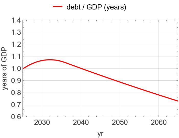
Debt-to-GDP ratio and deficit-to-GDP ratio achieved and improving.
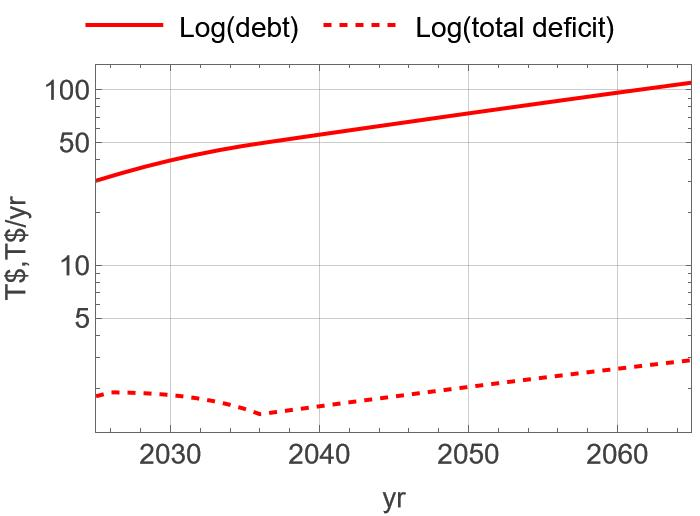
However, a falling debt-to-GDP ratio and deficit-to-GDP ratio are not a falling debt, deficit, nor interest; Debt × 3.6, deficit back to $2.9T, interest × 3.6”.
(1) “Reduce” the US deficits from 6% to 3% of GDP &
(2) “Stabilize” the U.S debt near 100% of GDP by 2036
Result:
Debt-to-GDP ratio and deficit-to-GDP ratio achieved and improving.
However, a falling debt-to-GDP ratio and deficit-to-GDP ratio are not a falling debt, deficit, nor interest; Debt × 3.6, deficit back to $2.9T, interest × 3.6”.
1. Introduction
1. Introduction
1.1. Debt, deficit, GDP, debt-to-GDP ratio, deficit-to-GDP ratio
1.1. Debt, deficit, GDP, debt-to-GDP ratio, deficit-to-GDP ratio
On 19 August 2026 the gross federal debt of the United States passed $40 trillion. It had reached $38 trillion the previous October and $39 trillion in March, a pace of roughly one trillion dollars every five months. The Congressional Budget Office (CBO) had projected the $40 trillion mark for 2027; it arrived a year early.The policy response most often proposed is to reduce the deficit. The Committee for a Responsible Federal Budget (CRFB) recommends cutting total deficits from about 6 percent of GDP to 3 percent by 2036, which it projects would hold debt near 100 percent of GDP (https://www.crfb.org/). Here is a statement by CRFB: The $40 trillion headline is gross debt, which includes roughly $8 trillion the government owes its own trust funds. Interest on that portion is paid by the government to itself and nets to zero in the unified budget. This model uses debt held by the public, $30.4 trillion at the close of FY2025, because that is the stock on which interest is actually paid. Multiplying gross debt by the average interest rate overstates net interest by about a quarter.

1.2. Objectives
1.2. Objectives
1.2.1. Debt-GDP dynamics
1.2.1. Debt-GDP dynamics
This notebook asks a narrow question. If that target is met in full, what happens to the debt and deficit?
I developed a System Dynamics model for the US federal debt-GDP dynamics; two stocks (Debt, GDP), three flows (primary spending, revenue, interest) and four parameters (interest rate r, economic growth g, spending share of GDP s(t), revenue share of GDP τ(t)). I achieved these two goals by reducing the government spending from 19.6% of GDP to 16.5% of GDP. Then it showed me something I did not expect: the debt-to-GDP ratio and deficit-to-GDP ratio are reduced but the debt continue to increase as well as the deficit. It is well known that stock-and-flow reasoning is where people frequently fail, and public debt & deficit are the simplest example I know of: reducing the deficit does not reduce the debt, the debt continue to grow but at slower rate.
I developed a System Dynamics model for the US federal debt-GDP dynamics; two stocks (Debt, GDP), three flows (primary spending, revenue, interest) and four parameters (interest rate r, economic growth g, spending share of GDP s(t), revenue share of GDP τ(t)). I achieved these two goals by reducing the government spending from 19.6% of GDP to 16.5% of GDP. Then it showed me something I did not expect: the debt-to-GDP ratio and deficit-to-GDP ratio are reduced but the debt continue to increase as well as the deficit. It is well known that stock-and-flow reasoning is where people frequently fail, and public debt & deficit are the simplest example I know of: reducing the deficit does not reduce the debt, the debt continue to grow but at slower rate.
1.2.2. Stock-and-flow and ratio structure
1.2.2. Stock-and-flow and ratio structure
My debt-GDP dynamic model reveals additional fact that a stock divided by a growing denominator or a ratio is another cognitive object that is difficult to comprehend (deficit-to-GDP ratio and debt-to-GDP ratio) and the vocabulary could mislead because “stabilized” might be heard as “stopped”. CRFB statement might give a rosy impression that the deficit and the debt will be reduced. However, a falling debt-to-GDP ratio and a falling deficit-to-GDP ratio are not a falling debt, deficit, nor interest bill. The debt will continue to increase as well as the deficit and interest. The reason is a stock-and-flow structure that is easy to state but difficult to reason about. Debt is a stock. The deficit is a flow into it. Reducing a flow (deficit) slows the growth of a stock (debt); it does not reduce the stock (debt). More importantly, debt carries a further complication that an ordinary stock does not: part of its inflow is interest, which is proportional to the stock itself.For any stock, level, or accumulation; dS/dt = inflow -outflow. Reducing the inflow reduces dS/dt, which is the rate of change, not the level. The stock only falls when inflow < outflow. So long as the inflow > outflow, the stock continues to rise -- more slowly, but it still rises. This is called error of correlation heuristic in System Dynamics; people assume the output of a system moves in the same direction as the input (e.g., Reducing CO2 emission will reduce CO2 in the atmosphere), which is only true for a flow-to-flow relationship, not for a flow-to-stock relationship.Here is the case with the debt-to-GDP ratio falls but the debt and deficit still rise. The debt and deficit are in log scale. , but
1.3. Debt-to-GDP Dynamics Model
1.3. Debt-to-GDP Dynamics Model
1.3.1. Two stock model
1.3.1. Two stock model
Here is a simplified model showing debt, primary spending, revenue, interest and GDP. Debt-to-GDP ratio and total deficit-to-GDP ration can be easily derived.
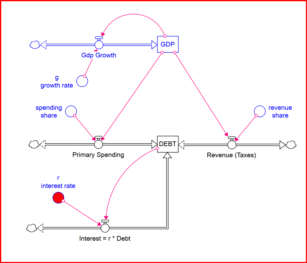
d(Debt)/dt=primaryspending+interest−revenue,d(GDP)/dt=g*GDP,
(
1
)primary spending = s (t) * GDP,
revenue = τ (t) * GDP,
interest = r * Debt .
The primary spending excludes net interest, which enters separately as r * Debt .
The primary balance = primary spending - revenue .
The primary deficit = revenue - primary spending .
If r*Debt is large relative to the primary balance, the debt can accelerate even when the primary deficit is driven to zero. Stabilization requires a primary surplus at least as large as r*D . In ratio terms, g > r . This is why the intuitive statement "we cut the deficit, so the debt problem is being solved" is structurally wrong .
revenue = τ (t) * GDP,
interest = r * Debt .
The primary spending excludes net interest, which enters separately as r * Debt .
The primary balance = primary spending - revenue .
The primary deficit = revenue - primary spending .
If r*Debt is large relative to the primary balance, the debt can accelerate even when the primary deficit is driven to zero. Stabilization requires a primary surplus at least as large as r*D . In ratio terms, g > r . This is why the intuitive statement "we cut the deficit, so the debt problem is being solved" is structurally wrong .
1.3.2. One stock model
1.3.2. One stock model
The two-stock system is reduced exactly into one dimensionless state variable. Let b = Debt/GDP = D/Y and pb = primary balance as a share of GDP. The quotient rule gives
db/dt=d(D/Y)/dt=(r−g)b−pb,pb=primarybalance/GDP
(
2
)Four quantities follow by inspection:
eigenvalue λ = r − g = −0.0060equilibrium b* = pb / (r − g)time constant τ = 1/|λ| = 167 yearsexact solution b(t) = b* + (b₀ − b*) exp(λt)If r < g, the D/Y ratio is drawn toward the resting point. Deficits are stable.If r > g, the D/Y ratio is pushed away from it. Deficits are not stable.Who or what organizations have control over the four parameters? Nothing in a tax bill changes the sign of (r − g). That sign is set by the central bank and by long-run productivity growth. So a government can move the target. It cannot decide whether the target holds. Right now the gap between those two worlds is about 60 basis points (r= 0.034, g = 0.040). One more thing, and it is uncomfortable. Cutting spending slows growth in the short run. Slower growth lowers g. Lower g pushes (r − g) toward the bad sign. The spending cut pushes the system the wrong way.The reduction itself is not new. That a growing economy stabilizes the debt ratio is Domar (1944); the modern form separating the primary balance from the interest term is standard in the IMF and CBO sustainability frameworks (Escolano 2010, equation 7, where the same quantity appears in discrete time as λ = (r−g)/(1+g)).
1.3.3. This model is calibrated for FY2025 actual values
1.3.3. This model is calibrated for FY2025 actual values
Debt held by the public $30.4 T Debt(2025)Nominal GDP $30.5 T GDP (2025)Revenue 17.1% of GDP $5.23T / $30.5TPrimary spending 19.6% of GDP ($7.01T − $1.02T) / $30.5TEffective interest rate 3.4% per year average on marketable debtNominal GDP growth 4.0% per year ~2% real plus ~2% inflation
1.3.4. The calibration reconciles with published FY2025 numbers
1.3.4. The calibration reconciles with published FY2025 numbers
total outlays my model $7.01T published $7.01Trevenue my model $5.22T published $5.23Tinterest my model $1.03T published $1.02Ttotal deficit my model $1.80T published $1.78Tdebt / GDP my model 1.00 published ~1.00Running one year forward yields a debt ratio of 101.6 percent for 2026, against CBO’s baseline figure of 101 percent. Total_Outlays = spending + Interest_Payments. Outlays simply means money actually paid out.
1.3.5. The policy scenario
1.3.5. The policy scenario
The consolidation reduces primary spending from 19.6 to 16.53 percent of GDP, linearly over 2026–2036, with revenue held at 17.1 percent. This is the spending-only route to the CRFB target. It is an adjustment of 3.07 percentage points of GDP, about $935 billion a year at FY2025 GDP. Two alternative routes reach the same target: revenue rising from 17.1 to 20.17 percent with spending unchanged, or a split of 1.53 points from each side. All three produce identical debt paths.
◼
Hit the goals: spending cut from 19.6% of GDP to 1%, holding the revenue share at 16.5% (i.e., no increase in taxes)
1.4. Simulation results
1.4. Simulation results
1.4.1 Outcomes from the spending cut policy
1.4.1 Outcomes from the spending cut policy
The target is met exactly. The total deficit reaches 3.00 percent of GDP in 2036.
year debt GDP debt/GDP interest deficit deficit
($T) ($T) (yr) ($T) ($T) (% GDP)
2025 30.40 30.50 1.00 1.03 1.80 5.89
2030 39.71 37.25 1.07 1.35 1.82 4.90
2036 49.66 47.36 1.05 1.69 1.42 3.00
2045 64.09 67.88 0.94 2.18 1.58 2.64
2065 110.20 151.07 0.73 3.75 2.89 1.91
($T) ($T) (yr) ($T) ($T) (% GDP)
2025 30.40 30.50 1.00 1.03 1.80 5.89
2030 39.71 37.25 1.07 1.35 1.82 4.90
2036 49.66 47.36 1.05 1.69 1.42 3.00
2045 64.09 67.88 0.94 2.18 1.58 2.64
2065 110.20 151.07 0.73 3.75 2.89 1.91
1.5. Surprising findings and conclusion
1.5. Surprising findings and conclusion
The debt never falls.
Over forty years it grows from $30.4 trillion to $110.2 trillion, a factor of 3.6, and it does not decline in a single year of the run. The interest bill grows by the same factor, from $1.03 trillion to $3.75 trillion. Nothing is repaid. The debt is diluted by a growing economy, not reduced.
The same pattern appears in the deficit.
In dollars, the deficit reaches its minimum of $1.42 trillion in 2036 — the very year the target is met — and then doubles to $2.89 trillion by 2065. As a share of GDP it falls falls steadily after 2026 to 1.91 percent. Both statements describe the same run. The share is the quantity that is targeted, reported and celebrated; the dollars are what has to be borrowed.
Interest is not a budget item
Everyone knows the interest bill passed $1 trillion. Congress votes on budget items such as defense, Medicaid, etc. However, interest is different. It is calculated, and the government has to pay it. There is a self-reinforcing loop. Debt creates interest. Interest is borrowed. Borrowing adds to debt. The deficit and debt are the part we argue about. Interest is the part that grows while we argue. The debt ratio falls while the debt triples. There are only two ways out. Grow faster than the interest rate, or run a surplus large enough to shrink the debt itself. The United States has not done the second since 2001.
Meeting a 3 percent deficit requires a primary surplus.
At 2036 interest alone is 3.57 percent of GDP, larger than the entire deficit target. The consolidation works only because it produces a primary surplus of 0.57 percent of GDP that partly offsets the interest bill. Hitting a 3 percent deficit does not mean spending 3 percent more than you collect; it means collecting more than you spend and still borrowing 3 percent because of interest owed on past borrowing.
Balancing the primary budget does not stop the growth.
If the primary deficit is driven to exactly zero — spending share equal to revenue share — the debt still grows from $30.4 trillion to $136.7 trillion over forty years, a factor of 4.5, because the remaining inflow is r × Debt and feeds on the stock it fills. An ordinary stock with its inflow reduced to zero would stop rising. Debt does not.
The model cannot distinguish a spending cut from a tax increase.
The three routes to the target give identical debt paths to four decimal places, because only the difference between the two shares enters the equation. Everything separating them — incidence, feasibility, the distribution of losses — lies outside the model.
Policy sets the position, not the stability.
In db/dt = (r−g)b − pb, the primary balance enters additively and relocates the equilibrium. The sign of (r−g) determines whether that equilibrium attracts or repels, and no fiscal measure changes it. A legislature controls pb directly. No one controls r or g: the central bank moves overnight rates, markets set long yields, the average rate on existing debt lags by roughly its maturity, and growth depends on productivity and demographics. The gap between a stable and an unstable regime is currently 0.6 percentage points, smaller than the error in any growth forecast.
What “3%” in spending cut actually costs
The spending cut I simulated is a delta of 3% of GDP, which seems a trivial amount, 3 out of 100. But it is not. The 3% of GDP is $935B dollars. The $935B is more than the entire defense budget ($804B). About the same as all of Medicare ($955B). Roughly everything the federal government spends on education, transportation, science, courts, national parks, veterans’ hospitals and air traffic control, combined. The The $945B about $7,000 per American households, every year.
“Cut spending by 3% of GDP” and “Raise taxes by 3% of GDP” describe the same amount of money: $935B dollars. Government primary spending is 19% of GDP. Cutting it from 19% to 16% of GDP removes 3 percentage points of the economy. But measured against the spending itself, 3 out of 19 is “one dollar in every six”.
A family earns $100,000 and spends $19,000 on food. Someone proposes cutting food spending by “3% of income.” That sounds like nothing. However, it is $3,000 off a $19,000 grocery budget. They have lost a sixth of what they eat.
Revenue is 17.1% of GDP. Raising it 3 points means collecting 18% more tax. If it all came from income tax, income tax collections would rise about 40%.
And here is the part that still surprises me. Even with the spending cut, spending never falls. It goes from $6 trillion in 2026 to $25 trillion over forty years. The economy grows underneath it, so a smaller slice of a bigger pie is still more pie.
A debt-to-GDP ratio that improves by 27 percent is consistent with a debt that more than triples and an interest bill that triples with it. The two statements are not in tension; they are the same arithmetic seen through different denominators. The word “stabilized” is doing the damage. In fiscal usage it does not mean the debt stops growing. It means the debt grows no faster than the economy. Those are very different claims, and the vocabulary conceals the difference.
The same confusion appears three times in this one model, at three different levels: in the policy input, where a cut of three percentage points of GDP is a cut of one dollar in every six of spending; in the flow, where the deficit share falls while the deficit in dollars doubles; and in the stock, where the ratio improves while the debt triples. The failure is not specific to public debt. It arises whenever a quantity is normalized by a growing denominator, and the direction of the error depends only on which denominator the speaker has chosen.
Two caveats. The model has no distributional content: one implicit representative household, no cohorts, no income deciles. It can size the required adjustment; it cannot say who should bear it. And it is not a forecast. It reconciles with FY2025 actuals and reproduces CBO’s 2026 debt ratio, but agreement at the initial date is calibration, not validation.
Over forty years it grows from $30.4 trillion to $110.2 trillion, a factor of 3.6, and it does not decline in a single year of the run. The interest bill grows by the same factor, from $1.03 trillion to $3.75 trillion. Nothing is repaid. The debt is diluted by a growing economy, not reduced.
The same pattern appears in the deficit.
In dollars, the deficit reaches its minimum of $1.42 trillion in 2036 — the very year the target is met — and then doubles to $2.89 trillion by 2065. As a share of GDP it falls falls steadily after 2026 to 1.91 percent. Both statements describe the same run. The share is the quantity that is targeted, reported and celebrated; the dollars are what has to be borrowed.
Interest is not a budget item
Everyone knows the interest bill passed $1 trillion. Congress votes on budget items such as defense, Medicaid, etc. However, interest is different. It is calculated, and the government has to pay it. There is a self-reinforcing loop. Debt creates interest. Interest is borrowed. Borrowing adds to debt. The deficit and debt are the part we argue about. Interest is the part that grows while we argue. The debt ratio falls while the debt triples. There are only two ways out. Grow faster than the interest rate, or run a surplus large enough to shrink the debt itself. The United States has not done the second since 2001.
Meeting a 3 percent deficit requires a primary surplus.
At 2036 interest alone is 3.57 percent of GDP, larger than the entire deficit target. The consolidation works only because it produces a primary surplus of 0.57 percent of GDP that partly offsets the interest bill. Hitting a 3 percent deficit does not mean spending 3 percent more than you collect; it means collecting more than you spend and still borrowing 3 percent because of interest owed on past borrowing.
Balancing the primary budget does not stop the growth.
If the primary deficit is driven to exactly zero — spending share equal to revenue share — the debt still grows from $30.4 trillion to $136.7 trillion over forty years, a factor of 4.5, because the remaining inflow is r × Debt and feeds on the stock it fills. An ordinary stock with its inflow reduced to zero would stop rising. Debt does not.
The model cannot distinguish a spending cut from a tax increase.
The three routes to the target give identical debt paths to four decimal places, because only the difference between the two shares enters the equation. Everything separating them — incidence, feasibility, the distribution of losses — lies outside the model.
Policy sets the position, not the stability.
In db/dt = (r−g)b − pb, the primary balance enters additively and relocates the equilibrium. The sign of (r−g) determines whether that equilibrium attracts or repels, and no fiscal measure changes it. A legislature controls pb directly. No one controls r or g: the central bank moves overnight rates, markets set long yields, the average rate on existing debt lags by roughly its maturity, and growth depends on productivity and demographics. The gap between a stable and an unstable regime is currently 0.6 percentage points, smaller than the error in any growth forecast.
What “3%” in spending cut actually costs
The spending cut I simulated is a delta of 3% of GDP, which seems a trivial amount, 3 out of 100. But it is not. The 3% of GDP is $935B dollars. The $935B is more than the entire defense budget ($804B). About the same as all of Medicare ($955B). Roughly everything the federal government spends on education, transportation, science, courts, national parks, veterans’ hospitals and air traffic control, combined. The The $945B about $7,000 per American households, every year.
“Cut spending by 3% of GDP” and “Raise taxes by 3% of GDP” describe the same amount of money: $935B dollars. Government primary spending is 19% of GDP. Cutting it from 19% to 16% of GDP removes 3 percentage points of the economy. But measured against the spending itself, 3 out of 19 is “one dollar in every six”.
A family earns $100,000 and spends $19,000 on food. Someone proposes cutting food spending by “3% of income.” That sounds like nothing. However, it is $3,000 off a $19,000 grocery budget. They have lost a sixth of what they eat.
Revenue is 17.1% of GDP. Raising it 3 points means collecting 18% more tax. If it all came from income tax, income tax collections would rise about 40%.
And here is the part that still surprises me. Even with the spending cut, spending never falls. It goes from $6 trillion in 2026 to $25 trillion over forty years. The economy grows underneath it, so a smaller slice of a bigger pie is still more pie.
A debt-to-GDP ratio that improves by 27 percent is consistent with a debt that more than triples and an interest bill that triples with it. The two statements are not in tension; they are the same arithmetic seen through different denominators. The word “stabilized” is doing the damage. In fiscal usage it does not mean the debt stops growing. It means the debt grows no faster than the economy. Those are very different claims, and the vocabulary conceals the difference.
The same confusion appears three times in this one model, at three different levels: in the policy input, where a cut of three percentage points of GDP is a cut of one dollar in every six of spending; in the flow, where the deficit share falls while the deficit in dollars doubles; and in the stock, where the ratio improves while the debt triples. The failure is not specific to public debt. It arises whenever a quantity is normalized by a growing denominator, and the direction of the error depends only on which denominator the speaker has chosen.
Two caveats. The model has no distributional content: one implicit representative household, no cohorts, no income deciles. It can size the required adjustment; it cannot say who should bear it. And it is not a forecast. It reconciles with FY2025 actuals and reproduces CBO’s 2026 debt ratio, but agreement at the initial date is calibration, not validation.
2. Debt-GDP Model: Two-stock model
2. Debt-GDP Model: Two-stock model
2.1. Revenue and Spending policy
2.1. Revenue and Spending policy
2.1.1. FY2025 actual values
2.1.1. FY2025 actual values
2.1.2. Define the spending & revenue path, spending cut starting in 2026 over 10 years.
2.1.2. Define the spending & revenue path, spending cut starting in 2026 over 10 years.
2.1.3. Display the spending and revenue path. We can simulate different paths: revenue increase, or even spending cut & revenue increase
2.1.3. Display the spending and revenue path. We can simulate different paths: revenue increase, or even spending cut & revenue increase
2.2. Debt-GDP Model
2.2. Debt-GDP Model
2.3. Debt-GDP Model Simulator
2.3. Debt-GDP Model Simulator
3. Debt-GDP Model: One-stock model
3. Debt-GDP Model: One-stock model
References
References
Domar, E. D. (1944). The burden of the debt and the national income. American Economic Review, 34(4), 798–827.
Escolano, J. (2010). A practical guide to public debt dynamics, fiscal sustainability, and cyclical adjustment of budgetary aggregates. IMF Technical Notes and Manuals 10/02.
Committee for a Responsible Federal Budget. The Debt Fixer. crfb.org/debtfixerWIP
CITE THIS NOTEBOOK
CITE THIS NOTEBOOK
US debt-GDP dynamics: why a stabilizing ratio still means a tripling debt
by Sangdon Lee
Wolfram Community, STAFF PICKS, September 15, 2026
https://community.wolfram.com/t/28015
by Sangdon Lee
Wolfram Community, STAFF PICKS, September 15, 2026
https://community.wolfram.com/t/28015