Athanasios Paraskevopoulos
Plotting basics encompass understanding and creating visual representations of mathematical functions. Essential functions include linear, quadratic, cubic, exponential, logarithmic, and trigonometric. Accurate plotting helps visually interpret relationships, trends, and predictions.
Introduction
Introduction
In this project, we will explore the fundamentals of plotting basic functions. This includes understanding the nature and types of these functions, such as linear, quadratic, exponential, and trigonometric, and visually representing them in a graphical form. The project will allow us to delve into the relationships between inputs and outputs, as well as the importance of selecting suitable scales for the axes. Through this, we’ll develop a solid foundation in mathematical graphing, a skill integral to many fields such as physics, engineering, economics, and data analysis. Let’s dive into the fascinating world of functions and their graphical representations.
Plotting Functions
Plotting Functions
In[]:=
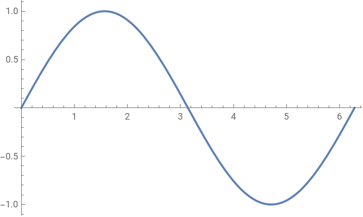
Plot[Sin[x],{x,0,2Pi}]
Out[]=
In[]:=
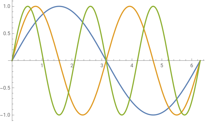
Plot[{Sin[x],Sin[2x],Sin[3x]},{x,0,2Pi},PlotLegends->Placed["Expressions",Below]]
Out[]=


In[]:=
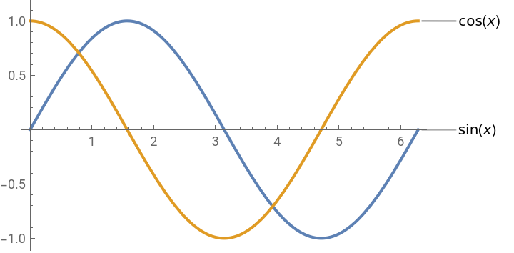
Plot[{Sin[x],Cos[x]},{x,0,2Pi},PlotLabels->"Expressions"]
Out[]=
Filling between two curves
Filling between two curves
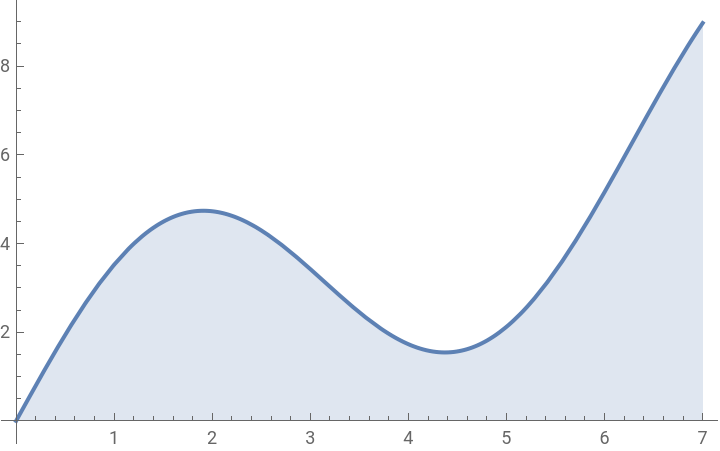
Let’s plot “” where is in range of 0 to 7 and filling the bottom
3sinx+x
x
In[]:=
Plot[3Sin[x]+x,{x,0,7},Filling->Bottom]
Out[]=
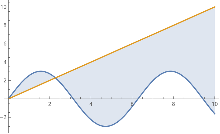
Plotting and filling between the curves and , where is in range of 0 to 10
sinx
x
x
In[]:=
Plot[{3Sin[x],x},{x,0,10},Filling->{1->{2}}]
Out[]=
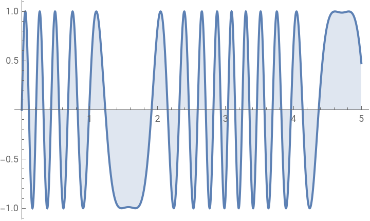
Plot the function , where is in range of 0 to 5
sin(30sin(x))
x
In[]:=
Plot[Sin[30Sin[x]],{x,0,5},Filling->Axis]
Out[]=
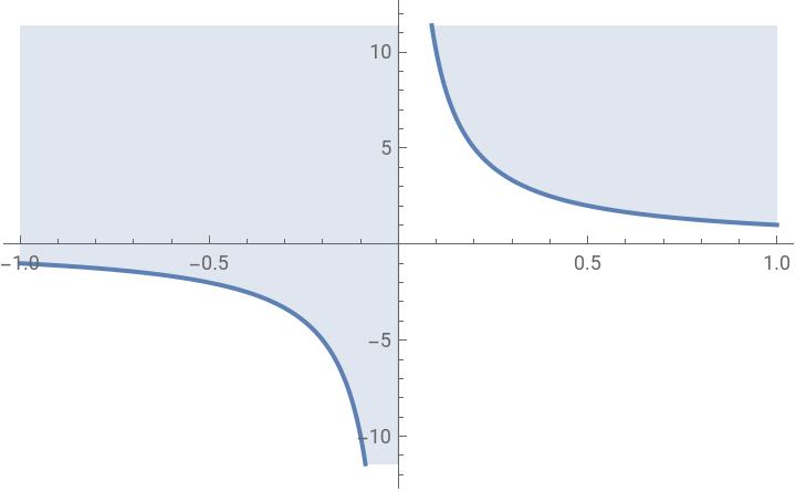
Plotthefunction,whereisinrangeof-1to1
1
x
x
In[]:=
Plot[1/x,{x,-1,1},Filling->Top]
Out[]=
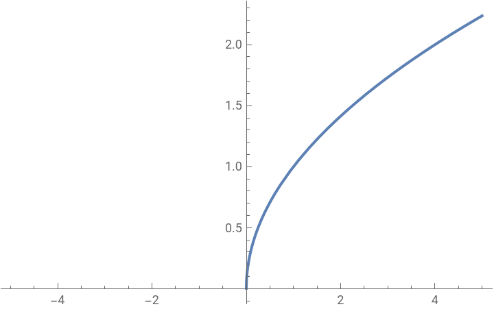
Drawing curves where function ranges becomes non reals, discontinuous and use of exclusion
Drawing curves where function ranges becomes non reals, discontinuous and use of exclusion
In[]:=
Plot[Sqrt[x],{x,-5,5}]
Out[]=
In[]:=
Plot[Floor[Sqrt[x]],{x,0,100}]
Out[]=
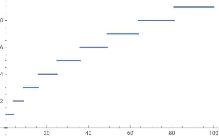
The Exclusions option in the Plot function is used to specify where Mathematica should leave breaks in the plot. This is typically useful when dealing with functions that have discontinuities, singularities, or other points where the function does not provide a real - valued output .
In this case, Mathematica will not exclude any points, and the plot may have a vertical asymptote
Labelling and Legending Curves
Labelling and Legending Curves
References
References
◼
Wolfram Mathematica Documentation Center - Plotting Guide:
https://reference.wolfram.com/language/guide/PlottingAndGraphics.html
https://reference.wolfram.com/language/guide/PlottingAndGraphics.html
◼
Wolfram Language & System Documentation Center - Plot function:
https://reference.wolfram.com/language/ref/Plot.html
https://reference.wolfram.com/language/ref/Plot.html
◼
Wolfram Alpha Blog - Advanced Plotting with Mathematica:
http://blog.wolframalpha.com/2011/06/28/advanced-plotting-with-mathematica/
http://blog.wolframalpha.com/2011/06/28/advanced-plotting-with-mathematica/
◼
Trott, M. (2004). The Mathematica GuideBook for Graphics. Springer-Verlag New York.