Domain walls are soliton topological defects believed to have occurred in the early universe during phase transitions [1]. These objects separate patches of space with different vacuum expectation values resulting from the spontaneously broken symmetry of an underlying potential. Domain walls contribute significantly to the energy density of the universe and must be considered when constructing cosmological models involving SSB [2]. In this project, our aim is to explore the possibility of similar behavior in graphs. We will implement methods for merging different graphs with wall-like structures and attempt to create an algorithm capable of finding them. Additionally, we will investigate the behavior of introduced domain walls while evolving the merged graphs.
1. Merging
1. Merging
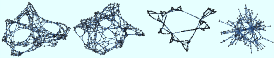
To begin the project we must first implement a method of merging two different graphs. In our search for “domain wall”-like behavior, we (obviously) want to point at some structure within the merged graph and identify it as the wall. In that case, the most natural approach seems to be choosing some vertices that belong to different graphs and introducing a trans-graph edge connecting them. At this point, we can state the first question of our post. How should we pick the vertices?Let us first define our well-behaved test subjects:
In[]:=
graph1=ResourceFunction["HypergraphToGraph"][ResourceFunction["WolframModel"][{{x,y},{x,z}}->{{x,z},{x,w},{y,w},{z,w}},{{0,0},{0,0}},10,"FinalState"]];graph2=ResourceFunction["HypergraphToGraph"][ResourceFunction["WolframModel"][{{x,y},{x,z}}->{{x,y},{x,w},{y,w},{z,w}},{{0,0},{0,0}},10,"FinalState"]];graph3=ResourceFunction["HypergraphToGraph"][ResourceFunction["WolframModel"][{{{1,2},{1,3}}->{{2,4},{2,4},{1,4},{3,1}}},{{0,0},{0,0}},10,"FinalState"]];graph4=ResourceFunction["HypergraphToGraph"][ResourceFunction["WolframModel"][{{{1,2},{1,3},{1,4}}->{{5,2},{2,5},{5,3},{3,4},{4,2}}},{{0,0},{0,0},{0,0}},17,"FinalState"]];Row[{graph1,graph2,graph3,graph4}]
Out[]=
1.1. Random merging
1.1. Random merging
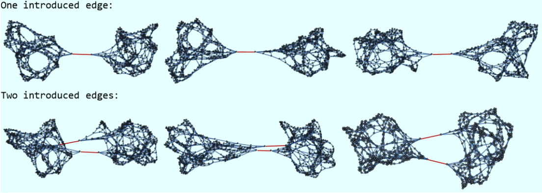
The easiest approach is to pick a number of vertices at random, from both graphs and insert the edges without troubling ourselves with insignificant matters such as the physical meaning of the method or the logic behind it. The following code does exactly that, introducing a number of edges defined by the parameter numofrel. All new edges are being highlighted on the newly merged graph.
randomMerg code shorcut
The results of such an operation differ from every calling of the function. Here we show three exemplary mergings for one and two introduced edges respectively.
Out[]=
1.2. Lowest Hausdorff dimension merging
1.2. Lowest Hausdorff dimension merging
Let us now assume that there exists a reader to whom the previous method will not be satisfactory and who will require the process to have some meaning instead (ridiculous, I know). To meet the expectations of such person we introduce a more deterministic procedure. In a directed graph one can estimate the Hausdorff dimension [3] around each vertex, which corresponds to local dimensionality. We can then pick the vertex with the lowest Hausdorff dimension and interpret it as the edge of space region described by our graph. In the following code, we implement this method and we pick the directions of new edges at random. One could also allow the new edges to be directed uniformly (graph1->graph2). This approach will be discussed in chapter 2.2. but for now let us restrict ourselves to the general method.
hausdorffMerg code shortcut
This method always yields the same result. Here we display an exemplary merging for 3, 9 and 16 artificially introduced edges.
Out[]=
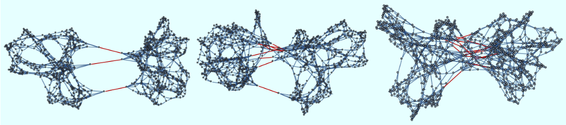
Looking at these examples we can already tell that the domains become visually less distinctive as the number of connections grows.
2. Recognition algorithm
2. Recognition algorithm
Now that we have a method of implementing artificial domain walls, we should also develop a tool that will allow us to find them. In a perfect world, such a tool should be able not only to point at the location of the domain boundaries but also tell whether they’re even there. In this section, we go over different approaches that we have tried and finally describe the one that worked.
2.1. Adjacency matrices
2.1. Adjacency matrices
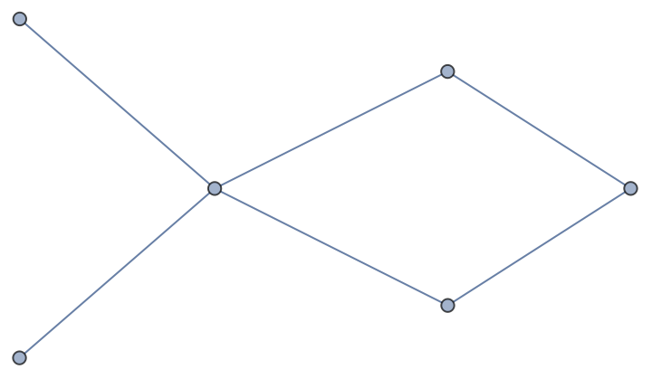
The working algorithm analyzes the adjacency matrix of a given graph. The adjacency matrix of a graph with n vertices is a matrix with elements defined as =1 if vertices and are adjacent and 0 else.
nn
a
ij
a
ij
v
i
v
j
a
ij
Out[]=
⧦
0 | 1 | 0 | 1 | 0 | 0 |
1 | 0 | 1 | 0 | 0 | 0 |
0 | 1 | 0 | 1 | 1 | 1 |
1 | 0 | 1 | 0 | 0 | 0 |
0 | 0 | 1 | 0 | 0 | 0 |
0 | 0 | 1 | 0 | 0 | 0 |
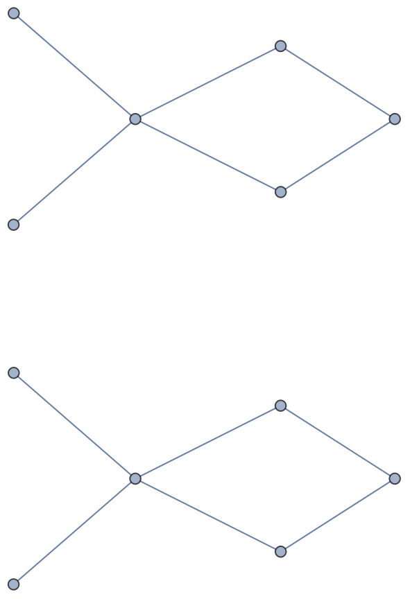
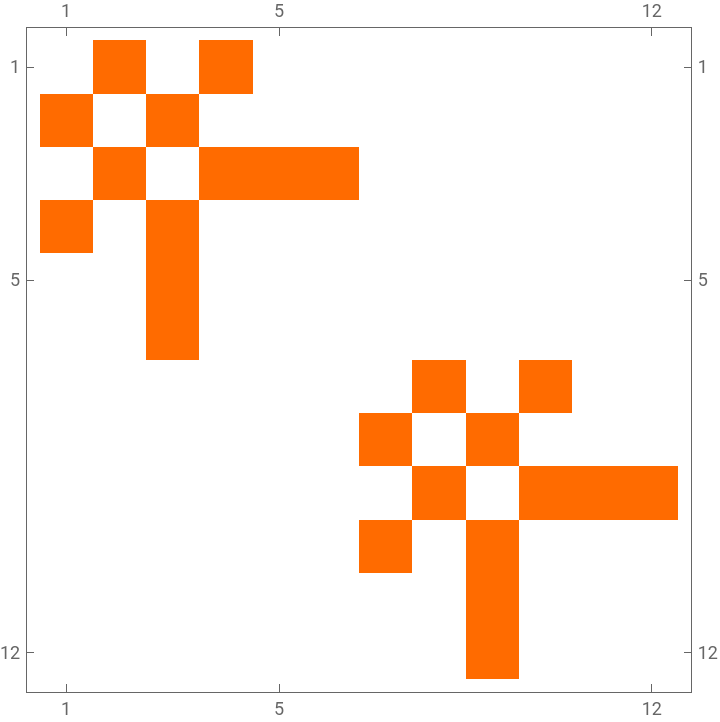
One of the properties of such matrices is crucial to our search. The adjacency matrix of two disconnected graphs can be divided into four “bins”, two of which consist of only zeros and the other two describe all the connections within each disconnected graph.
Out[]=
0 | 1 | 0 | 1 | 0 | 0 | 0 | 0 | 0 | 0 | 0 | 0 |
1 | 0 | 1 | 0 | 0 | 0 | 0 | 0 | 0 | 0 | 0 | 0 |
0 | 1 | 0 | 1 | 1 | 1 | 0 | 0 | 0 | 0 | 0 | 0 |
1 | 0 | 1 | 0 | 0 | 0 | 0 | 0 | 0 | 0 | 0 | 0 |
0 | 0 | 1 | 0 | 0 | 0 | 0 | 0 | 0 | 0 | 0 | 0 |
0 | 0 | 1 | 0 | 0 | 0 | 0 | 0 | 0 | 0 | 0 | 0 |
0 | 0 | 0 | 0 | 0 | 0 | 0 | 1 | 0 | 1 | 0 | 0 |
0 | 0 | 0 | 0 | 0 | 0 | 1 | 0 | 1 | 0 | 0 | 0 |
0 | 0 | 0 | 0 | 0 | 0 | 0 | 1 | 0 | 1 | 1 | 1 |
0 | 0 | 0 | 0 | 0 | 0 | 1 | 0 | 1 | 0 | 0 | 0 |
0 | 0 | 0 | 0 | 0 | 0 | 0 | 0 | 1 | 0 | 0 | 0 |
0 | 0 | 0 | 0 | 0 | 0 | 0 | 0 | 1 | 0 | 0 | 0 |
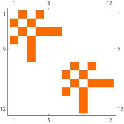
Let us now examine the adjacency matrices of merged graphs. From now on we will work with SparseArrays and use MatrixPlot to visualize our arrays.
Out[]=
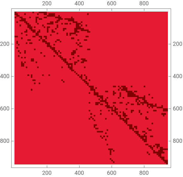
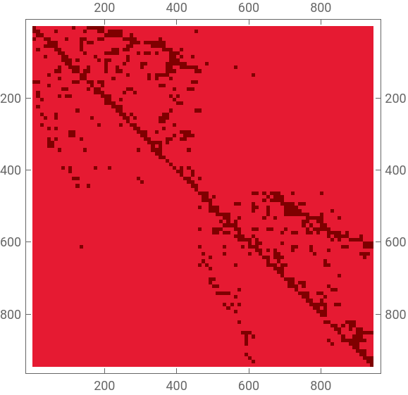
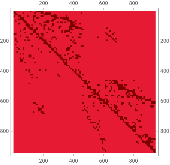
In the first matrix, not much can be seen. As expected, one can tell that there are bins with only zero elements. In the second matrix (5 connections) we begin to notice elements appearing in previously empty regions. These elements correspond to edges artificially introduced by hausdorffMerg. In the last matrix (45 connections) we can see that clearly. The methods that we will present work under a strong assumption. One inconvenient property of adjacency matrices is that they are not invariant under a permutation of indices of the vertices, even though the graphs’ geometry remains the same. For example, here we display the adjacency matrices of the same graph, which differ only by vertex indexing:
Out[]=
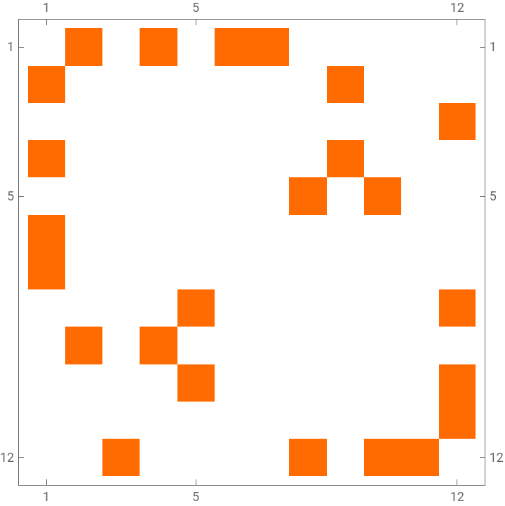
As we can see, the second matrix loses all previously discussed properties. Thus the Adjacency Matrix approach is only going to be valid for graphs that were indexed when separate and then artificially merged. One might think that having such information, the algorithm is going to be trivial, however, it is important to remember that we are not assuming anything about the subgraph matrices, only that they used to be there. Another obstacle lies in the fact that we have no way of telling where the subgraph matrices end and the artificial edges begin.
The physical meaning of this scenario is not without reason either. Real-world domain walls used to appear spontaneously between regions of space, whenever the early universe underwent a phase transition [2]. These objects would then become stable and divide patches of different vacuum expectation values. In other words, the idea of disconnected regions, patched by “unnatural” structures is not completely unrelated to physics.
The physical meaning of this scenario is not without reason either. Real-world domain walls used to appear spontaneously between regions of space, whenever the early universe underwent a phase transition [2]. These objects would then become stable and divide patches of different vacuum expectation values. In other words, the idea of disconnected regions, patched by “unnatural” structures is not completely unrelated to physics.
We are now ready to start discussing the algorithms. Let us begin with the previously dismissed case of introducing edges with uniform direction (section 1.1.). In this example, all artificial edges lie in one bin; either top right or bottom left. The detection algorithm is then very simple; -We check what’s the largest bin in the matrix which contains only zeros-We perform a reflection of the bin by the middle point of the matrix-We find points lying in the newly obtained bin, which are exactly the “domain wall” edgesThe process illustrated on a 1-connection matrix looks as follows:
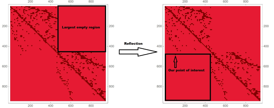
We can now see that, even though a human might find it hard to spot the connection, our robust algorithm handles it quite easily. Sadly, this procedure is not general, nor is it free of defects. An exemplary defect can be described as follows. Let us consider a merged graph consisting of two connected graphs. One of them could yield an adjacency matrix so asymmetrical, that (even though it would still be contained by a square) our procedure would overgrow the empty region bounds and have it flow into the graph-containing square. Going forward with the algorithm, the reflected region would now flow into the square from the other side, however, due to the asymmetry it could now pick up points corresponding to natural edges.
In general, the most obvious downside to such a method is the assumption of uniform direction of artificial edges. Without it, the algorithm cannot define a region to look into and breaks completely. Since no compelling argument was found for our domain walls to behave this way, we must continue our search.
In general, the most obvious downside to such a method is the assumption of uniform direction of artificial edges. Without it, the algorithm cannot define a region to look into and breaks completely. Since no compelling argument was found for our domain walls to behave this way, we must continue our search.
2.2. Final algorithm
2.2. Final algorithm
It is clear that such a matrix consists not of two but three bins containing non-zero values, describing the graphs. Should we then start implementing more algorithms to search for more than two domains? Not necessarily. All we have to do is apply our procedure to the subgraphs that were found the first time. Once we cannot identify any more connections; the process is complete.
At this point methodology ends and troubleshooting begins.
At this point methodology ends and troubleshooting begins.
As displayed in the cell above, the algorithm won’t search for more than 15 artificial edges unless it is specifically told to do so. Thus the first calling fails but the second succeeds.
Let us explore its limitations. In the cells below we display the results of running the algorithm on graphs merged with 30, 50 and 80 edges respectively.
Let us explore its limitations. In the cells below we display the results of running the algorithm on graphs merged with 30, 50 and 80 edges respectively.
With that many edges, we can no longer visually tell if we succeeded, however after a quick re-writing of our algorithm (modify to return disjoint subgraphs instead), we get:
We can see that the algorithm managed to find 80 artificial edges correctly and broke down at a hundred. Considering that our exemplary graphs consist of around 450 vertices each, that is not a bad score.
2.3. Registry of failed attempts
2.3. Registry of failed attempts
Geodesic ball intersection
Geodesic ball intersection
Growth acceleration of the volume
Growth acceleration of the volume
3. Evolution of domain walls
3. Evolution of domain walls
We have investigated methods of introducing domain walls and we’ve semi-successfully attempted to create a tool for finding them. All that is left is to explore their future. Even though we have developed methods of merging graphs arising from different rewriting rules, it is not so trivial to make an argument for a particular way of continuing their lifespan. After all, should we apply the rules used to develop the first subgraph? Should it be the rules of the second? Or maybe both? These questions do not seem to have a correct answer and our choice becomes arbitrary. One way of avoiding such ambiguities is to limit ourselves to cases that favor only one natural way of thought.
3.1 Graphs arising from one set of rewriting rules
3.1 Graphs arising from one set of rewriting rules
In this section we will shortly explore the evolution of graphs emerging from the same set of rewriting rules, but with different initial conditions. Let us define our test subjects. We will start with graphs emerging at earlier steps so that our notebooks can evaluate in finite time when evolving them later on.
Merging the two (hausdorffMerg) with a couple numbers of introduced edges:
Let us now perform a few steps of evolution for each merged graph, applying their original rule.
Evolutions depicted in the cell above look quite similar to the ones obtained through vertex-producing rules. We can see that the points that began their journey at the boundaries of the domain walls, migrate around the graph with different dispersion in each evolution path.
3.2. Hyperbolic surface graphs
3.2. Hyperbolic surface graphs
We perform merging of the two using randomMerg, since hausdorffMerg requires the graphs to be directed. We will touch on the reasoning behind this method shortly.
We pick a set of rules and evolve the graphs a few times, using “WolframModel” resource function. We highlight the points which encapsulated the initial domain wall and we follow them through each time step.
As we can notice in step 4, one of the points has migrated to the middle of one of the clusters. We observe the two subgraphs to become less visually distinctive and thus we conclude that this particular set of graphs and rules dissipates the domain wall. Let us now wonder if conclusions obtained in this manner are general to their respective cases. The sprinkling on hyperbolic surfaces is done using the Poisson process [5], meaning that every calling of the three cells above will yield a different result. For that reason, using randomMerg is not causing much damage to the reasoning behind this experiment. In general, for some set of rules, it might even be possible to stumble upon sprinkling and/or merging that would yield a graph with domain walls behaving like an eigenstate of the chosen rules. Thus any conclusions made about the behavior of such objects will not only be rule dependent but will also vary between each evaluation.
Conclusions
Conclusions
Acknowledgements
Acknowledgements
I would like to thank our deputy dean Krzysztof Turzyński for the great effort he put into having sent the Polish IPT2023 team to Wolfram Summer School. I would also like to express my sincere gratitude to the legion of my mentors: Nikola Bukowiecka, Manojna Namuduri, Christopher Wolfram and Xerxes Arsiwalla for their invaluable help in choosing the project and seeing it through.
References
References
[1] Va. B. Zel’dovich, I. Yu. Kobzarev, and L. B. Okun (1974). Cosmological consequences of a spontaneous breakdown of a
discrete symmetry
[2] Lazarides, G., Shafi, Q., & Walsh, T. F. (1982). Cosmic strings and domains in unified theories. Nuclear Physics B, 195(1)
[3] https://www.wolframphysics.org/technical-introduction/limiting-behavior-and-emergent-geometry/the-notion-of-dimension/
[4] https://www.wolframphysics.org/technical-introduction/limiting-behavior-and-emergent-geometry/geodesics/
CITE THIS NOTEBOOK
CITE THIS NOTEBOOK
Domain walls in graphs
by Tomasz Mazur
Wolfram Community, STAFF PICKS, 13 July, 2023
https://community.wolfram.com/groups/-/m/t/2959971
by Tomasz Mazur
Wolfram Community, STAFF PICKS, 13 July, 2023
https://community.wolfram.com/groups/-/m/t/2959971