This notebook series is designed to introduce selected dynamic economic models to both advanced undergraduate and graduate students. Economists have relied on a series of economic models to better understand the otherwise highly complex causal relationship among many economic variables. Dynamic economic models set up by systems of either difference or differential equations are particularly useful in tracing the change in the quantity of unknown economic variables (e.g., the capital stock, demand for labor, aggregate output, etc.) and their interactions over time.
This notebook series aims to help students better understand the depth, usefulness, and limitations of major existing micro and macroeconomic models by demonstrating how we can use Wolfram Mathematica to replicate and reconstruct the core ideas and find dynamic solution of the model.
The model introduced in this notebook series include, among others, (1) the cobweb model of the quantity and price adjustment, (2) Keynes’s aggregate demand model, (3) Hicks’s ISLM model, (4) Samuelson’s investment accelerator model, (5) Kalecki’s investment delay model, (6) the predator-prey interaction model, (7) the epidemic model, (8) Ricardo’s three dimensional business cycle model, (9) Marx-Goodwin business cycle and growth model, (10) Smith’s and Ricardo’s growth model, (11) the Harrod-Domar growth model, (12) the Solow growth model, (13) the RBC model, (14) Romer’s new growth model, and (15) the circuit of capital model.
Introduction
Introduction
Economic growth is a complex phenomenon that involves a cumulative change in some crucial constituent variables . One famous British economist Nicholas Kaldor (1908-1986) once highlighted these cumulative changes in the name of 'stylized facts .' One important stylized fact of economic growth is the change in the capital - output ratio. As the economy grows, the rate of change in aggregate output relative to the change in the total capital stock tends to grow faster. The same is true for the capital - labor ratio. The economic growth typically involves the increasing ratio of the non - labor capital stock relative to the growth of the demand for human labor. The same economic growth process is also accompanied by a certain business cycle pattern. The growth process is neither smooth nor stable. Instead, even if the measured aggregate output seems to increase exponentially, it always exhibits recurrent fluctuations in this exponential growth trajectory. Finally, any growth process must induce a certain distributive outcome. The distribution of national income can be relatively even in some countries, while at the same time the inequality in income distribution can worsen depending on the social institution that a particular economic community under consideration relies on.
For the last several sessions, we have learned some important economic growth models presented and taught by many influential macroeconomists. These include Harrod-Domar growth model, the Solow growth model, the RBC model, and Romer’s new growth model. As a way of concluding our discussion of economic growth models, this notebook presents one alternative framework that can potentially incorporate both business cycle patterns with the economic growth process. This model can also explain the distribution of national income, as well. The model we discuss in this notebook is called the ‘circuit of capital model.’
One unique feature of this circuit of capital model is that it is based upon the commonsense idea that what economists call the ‘capital stock’ in fact can take many different forms: It can be a certain amount of money. This money, of course, can be a borrowed money (e.g., bank loan) or it can be a result of the past savings held by a new prospective business owner. Let us call this amount of money either borrowed or saved the financial capital stock. This financial capital stock will be used to finance the establishment and operation of a production facility (e.g., a factory and plant). Once this ‘investment’ spending happens, the business owner will begin to operate this production facility by purchasing and installing non-labor fixed capital stock and by hiring workers who would operate machine and equipment to produce the finished products. We can call the market value of this productive facility including hired workers the productive capital stock. The source of financing for this production activity must come from the initial expenditure of the financial capital stock. If the business owner manufactures and produces a certain quantity of finished products that are ready to be sold on the market, we can call this output the commercial capital stock. At a given point in time, the sum of the three forms of the capital stocks constitutes what economists call the total capital stock.
The circuit of capital model in this way is designed to identify the three forms of the capital stocks and their interactive relationships. One form of the capital stock must be successively transformed into another form, so that the business owner continue her business activity over time. If the business owner spends a greater amount of the financial capital stock, this investment spending will be accumulated over time in the form of the greater productive capital stock (‘productive capacity’), which, in turn, may contribute to the production of a greater quantity of finished products (‘inventory’) that will be transferred to the node of the commercial capital stock and the financial capital stock in order, assuming that they are sold on the market as intended. If this ‘expansionary’ process continues, the total capital stock will grow and accumulate, increasing the market value of the aggregate output-income in the economy as a whole. If the interaction among the three capital stocks is disrupted, for some reasons, then the economic growth process will also be negatively affected. In this way, the circuit of capital model provides a powerful ‘stock-flow consistent modeling framework’ with which we can identify the necessary condition for the reproduction and accumulation of the system.
In addition, with this circuit of capital model framework, we can directly determine the two different sources of income accruing to the business owner and their hired workers, respectively. The business owner spends her financial capital stock to purchase both labor and non-labor input. Total amount of the financial capital stock used to purchase the labor input will be the total labor income accrued to hired workers. Compared to the total labor income, the business income or the income accrued to the business owner must come from the sales of the finished products. The source of this profit income net of all the expenditure including the labor cost comes from the very production process in which a new value is generated. In accounting, this new value portion created in the production process and transferred to the commercial capital stock is called ‘value-added.’ In the original literature, it is also called ‘surplus value.’ The income for the business owner is then the realization of this surplus value that is generated and augmented in the prior production activity and that is contained in the unit of finished products. Out of this total surplus value, a portion will be used up by the business owner for her final consumption, and the remaining portion will be used to increase the financial capital stock for the next round of the circuit. How much of this realized surplus value is divided into the two purposes will determine the reproduction and accumulation of the existing circuit of capital. In this way, we can derive the capital income and labor income directly from the circuit of capital model framework without introducing and relying on any metaphysical hypothesis about income distribution such as the marginal productivity theory of income distribution.
In what follows, we present a baseline model of the circuit of capital and demonstrate how we can generate various simulation results based upon a series of plausible economic scenarios. Karl Marx originally proposed the circuit of capital model idea (1990, 1993), and it was later successively developed by many influential Marxian economists led by Foley (1986) and Basu (2011). Shin (2025) has also contributed to this analysis. Intrigued readers can find more detailed bibliography suggested in the reference section. The current notebook is based upon Shin (2025)’s recent computational work.
The model structure
The model structure
A diagram for the modified circuit of capital
A diagram for the modified circuit of capital
Let us start by drawing a diagram for this model. The financial capital stock is denoted by F(t), the productive capital stock by N(t), and the commercial capital stock by X(t). The three capital stocks are connected by the three flows, one financial capital outlays (C(t)), the second, the production and delivery of finished products (P(t)), and the last capitalization of the realized surplus value (S(t)). When the business owner engages in financial capital outlays, she divides the entire financial capital stock into either purchasing non-labor input or buying labor input. How much of the entire financial expenditure will be used to purchase either of these inputs will be determined by a technical composition parameter κ. When the business owner completes production and delivers finished products to the node of the commercial capital stock, there must be an augmented value, which is captured by another parameter q. When the same business owner completes her sales of the final goods, she will earn a certain revenue (or profit if it is subtracted by all the previous expenditure). This revenue is then divided by a capitalization ratio p that shows how much of newly generated business income is recommitted to the financial capital stock for the next round of the circuit and how much is used for the business owner’s final consumption. Notice that in all these flows, there are certain time delay variables: Tf is the time lag for mobilizing and spending the financial capital stock, Tp is the time lag tied up in the production process, and Tr is the time lag for selling the finished products and collecting sales revenue.
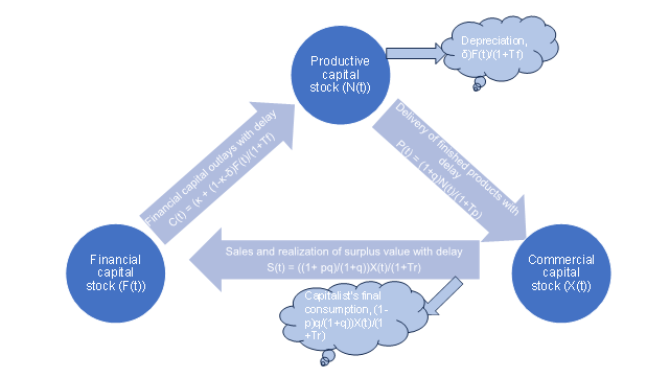
The structure of model
The structure of model
Mathematically, we can write the following system of three differential equations that represent this idea:
N
t
X
t
F
t
(
1
)LI[t]=(1-κ-δ)F(t)/(1+Tf)CIFC[t]=((1-p)q/(1+q))X[t]/(1+Tr)
(
2
)The productive capital stock (N(t)) is an increasing function of the expenditure of the financial capital stock (F(t)) and a decreasing function of the delivery of finished product to the node of the commercial capital stock (X(t)). The financial capital outlays consists of the two parts, one for buying non-labor input and the other for buying labor power. The exact proportion of this financial expenditure is determined by the parameter κ.
The financial capital stock is an increasing function of the inflow of sales revenue, which is determined by the surplus value q and the parameter p that determines how much of the realized surplus value is recommitted to augment the previous financial capital stock for the next round of the circuit. The higher value of p, the greater the financial capital stock in the next round of the circuit given q. Given p, the higher value of q also increases the financial capital stock in the successive round of the circuit.
In addition to these core stock and flow relationship, we can also derive the two variables that explain the change in labor income (LI(t)) and the capitalist income for final consumption (CIFC(t)). In this formulation, the total labor income is nothing more than the portion of the capitalist’s financial capital outlays that is used to purchase labor power, (1-κ-δ)F(t), adjusted by the corresponding time lag. That is, (1+Tf), (1-κ-δ)F (t)/(1+Tf). The capitalist income for final consumption is the portion of realized surplus value that is not recommitted to the next round of the circuit. That is, ((1-p)q/(1+q))X[t]/(1+Tr).
The simple reproduction of the model with and without time-lags
The simple reproduction of the model with and without time-lags
A simple reproduction without time-lags
A simple reproduction without time-lags
What will be the solution to this new system? As a starter, suppose that this system does not grow. In our model setup, this means that the circuit of capital merely reproduces itself at the existing scale of operation. Newly generated income or realized surplus value is entirely consumed by the capitalist-manufacturer-entrepreneur. In this case, the capitalization ratio will be zero (p = 0).
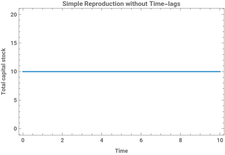
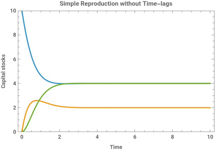
Let us also suppose that the three time lags are all zero (Tf = Tp = Tr = 0). If we further assume that the depreciation of the productive capital stock is negligible (δ = 0), the technical composition parameter, κ = 0.5, and the realized surplus value, q = 1, with initial value of the financial capital stock, F[0] = 10, while initial value of both the productive and commercial capital stock are all zero, N[0] = X[0] = 0, we can get the following simulation result:
In[]:=
Clear[eqns,sol,FCS,PCS,CCS,FCS0,PCS0,CCS0,sol,t,κ,δ,p,q];eqns={FCS'[t]==(1+p*q/(1+q))*CCS[t]-(κ+(1-κ-δ))*FCS[t],PCS'[t]==(κ+(1-κ-δ))*FCS[t]-(1+q)*PCS[t],CCS'[t]==(1+q)*PCS[t]-((1+(p*q)+(1-p)*q)/(1+q))*CCS[t],FCS[0]==FCS0,PCS[0]==PCS0,CCS[0]==CCS0};κ=0.5;δ=0.0;p=0.0;q=1;FCS0=10;PCS0=0;CCS0=0;sol=NDSolve[eqns,{FCS[t],PCS[t],CCS[t]},{t,0,100}];
In[]:=
Plot[Evaluate[FCS[t]+PCS[t]+CCS[t]/.sol],{t,0,10},Frame->True,FrameLabel->{"Time","Total capital stock"},PlotLabel->"Simple Reproduction without Time-lags",LabelStyle->Directive[Bold]]Plot[Evaluate[{FCS[t],PCS[t],CCS[t]}/.sol],{t,0,10},PlotRange->{0,10},PlotLegends->{"F(t)","N(t)","X(t)"},Frame->True,FrameLabel->{"Time","Capital stocks"},PlotLabel->"Simple Reproduction without Time-lags",LabelStyle->Directive[Bold]]Plot[Evaluate[{(1-κ-δ)*FCS[t],((1-p)*q/(1+q))*CCS[t]}/.sol],{t,0,10},PlotRange->{0,10},PlotLegends->{"LI(t)","CIFC(t)"},Frame->True,FrameLabel->{"Time","Two incomes"},PlotLabel->"Simple Reproduction without Time-lags",LabelStyle->Directive[Bold]]
Out[]=
Out[]=


Out[]=
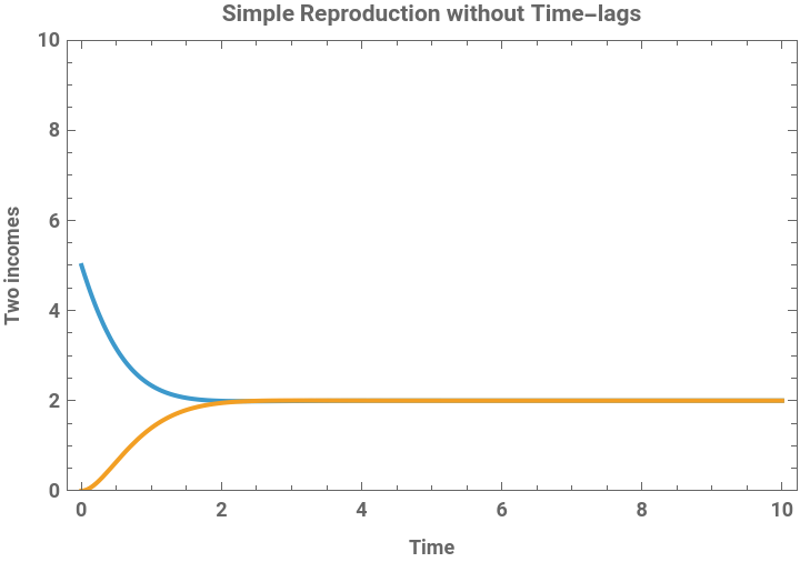
At the beginning, the financial capital stock decreases as it is used to set up and organize the production activity. The productive capital stock, in turn, initially increases and reaches its peak as more and more financial capital outlays are used to support it, but it decreases as finished products are delivered to the node of the commercial capital stock. The realized surplus value contained in the sales revenue leaks out from the circuit in the form of the capitalist’s income for final consumption. Therefore, the total capital stock, the sum of the three capital stocks remains the same as before (F[t]+N[t]+X[t] =10). The labor income falls from its initial value ((1-κ)F[0] = 0.5*10 = 5) and converges to the capitalist’s income for final consumption (LI[t] = CIFC[t] → 2).
A simple reproduction with time-lags: The case when Tf = Tp = Tc = 2
A simple reproduction with time-lags: The case when Tf = Tp = Tc = 2
Using the same parameter and initial values above, we can also run the simulation for the simple reproduction with some positive time-lags. Suppose first that the three time-lags are evenly increased from zero to two. That is, Tf = Tp = Tr = 2. We can also simulate the case when the three time-lags are changed unevenly, for example, by Tf = 2, Tp = 1, and Tr = 0.
If the three time-lags are evenly increased, the speed of the adjustment among the three capital stocks slows down proportionately. The speed of the distribution of the two social class incomes is also negatively affected in tandem by the evenly lengthened time-lags. The higher the value of the time-lags, the lower and slower the volume and accumulation of the three capital stocks.
In[]:=
Clear[eqns,sol,FCS,PCS,CCS,FCS0,PCS0,CCS0,Tc,Tf,Tp,sol,t,κ,δ,p,q];eqns={FCS'[t]==(1+p*q/(1+q))*CCS[t]/(1+Tc)-(κ+(1-κ-δ))*FCS[t]/(1+Tf),PCS'[t]==(κ+(1-κ-δ))*FCS[t]/(1+Tf)-(1+q)*PCS[t]/(1+Tp),CCS'[t]==(1+q)*PCS[t]/(1+Tp)-((1+(p*q)+(1-p)*q)/(1+q))*CCS[t]/(1+Tc),FCS[0]==FCS0,PCS[0]==PCS0,CCS[0]==CCS0};κ=0.5;δ=0.0;p=0.0;q=1;FCS0=10;PCS0=0;CCS0=0;Tp=2;Tf=2;Tc=2;sol=DSolve[eqns,{FCS,PCS,CCS},{t,0,100}];
In[]:=
Plot[Evaluate[FCS[t]+PCS[t]+CCS[t]/.sol],{t,0,10},Frame->True,FrameLabel->{"Time","Total capital stock"},PlotLabel->"Simple Reproduction with Time-lags",LabelStyle->Directive[Bold]]Plot[Evaluate[{FCS[t],PCS[t],CCS[t]}/.sol],{t,0,10},PlotRange->{0,10},PlotLegends->{"F(t)","N(t)","X(t)"},Frame->True,FrameLabel->{"Time","Capital stocks"},PlotLabel->"Simple Reproduction with Time-lags",LabelStyle->Directive[Bold]]Plot[Evaluate[{(1-κ-δ)*FCS[t]/(1+Tf),((1-p)*q/(1+q))*CCS[t]/(1+Tc)}/.sol],{t,0,10},PlotRange->{0,10},PlotLegends->{"LI(t)","CIFC(t)"},Frame->True,FrameLabel->{"Time","Two-class incomes"},PlotLabel->"Simple Reproduction with Time-lags",LabelStyle->Directive[Bold]]
A simple reproduction with time-lags: The case when Tf > Tp >Tc ≥ 0
A simple reproduction with time-lags: The case when Tf > Tp >Tc ≥ 0
In contrast, if any of the three time-lags is changed unevenly, the pattern of the interaction among the three capital stocks is fundamentally altered, so is the level and distribution of the two class incomes.
The expanded reproduction with uniform changes in time-lags
The expanded reproduction with uniform changes in time-lags
The expanded reproduction
The expanded reproduction
Let us now consider the behavior of the system under the assumption that the three capital stocks continue to grow as a greater amount of the realized surplus value is recommitted to the circuit. This continuous growth of the three capital stocks corresponds to expanded reproduction of capital.
This form of reproduction requires that the injection variable be always greater than sum of the two leakage variables, and, in our current model setting, it involves the increase in some crucial parameters, primarily the capitalization ratio, p, and/or the realized surplus value, q. This expanded reproduction is also affected by the potential change in any of the three time-lags.
For this analysis, however, we do not need to introduce any restrictive assumption such as the equi-proportional growth rate of the three capital stocks as assumed in Foley’s analytical solution. In this section, we assume for simplicity that there is no change in the three time-lags. Even when we begin to consider the effect of the change in time-lags, we will continue to assume that the three time-lags are uniformly changed in the same direction.
The effect of the change in the capitalization ratio
The effect of the change in the capitalization ratio
Let us first examine the effect of the changing capitalization rate, p, from 0.2 to 1.0 with an increment of 0.2 on the speed and level of the growth of the three capital stocks as well as on the two social class incomes, assuming that all other parameters and initial conditions remain the same as before. That is, N[0] = 0, X[0] = 0, F[0] = 10, and κ = 0.5, δ = 0.0, and q = 1. Suppose also that three time-lags are uniformly zero for the moment. That is Tp = Tf = Tr = 0.
Under this scenario, the simulation result shows that the increase in realized surplus value has a positive impact on the speed of the growth of the three capital stocks. Given the fixed realized surplus value, q = 1, a higher capitalization ratio means that a greater amount of the realized surplus is reinvested. The higher the value of this capitalization rate, p, the faster and the greater the growth of the three capital stocks. Consequently, we can also observe that the total capital stock grows faster with a higher capitalization ratio.
Similarly, the change in the capitalization rate affects the labor income proportionately. As the higher capitalization rate speeds up the accumulation of both the financial and productive capital stock, it increases the total demand for labor and/or labor income with a fixed technical composition ratio.
Compared to the labor income, however, the higher value of the capitalization rate is associated with the lower capitalist’s income for final consumption. If the capitalist-manufacturer-entrepreneur reinvests an increasing portion of the sales revenue to accumulate more and faster the productive capital stock, its residual, the capitalist’s income for final consumption leaked from the circuit must be smaller than otherwise. Therefore, there is an intertemporal tradeoff between the current and future final consumption for the capitalist induced by his decision over the capitalization rate.
The effect of the change in realized surplus value
The effect of the change in realized surplus value
We can find the same qualitative behaviors of the solution curves in the growth of the three capital stocks if we change the realized surplus value, q, from 0.2 to 1.0. Given the fixed capitalization ratio (p = 0.5), while assuming all other parameters and time-lags remain the same as before, a greater surplus value has a similar positive impact on the level and speed of the accumulation of the three capital stocks. The greater the value of this surplus value, the faster the growth of the three capital stocks. Therefore, the accumulation of the total capital stock is also directly affected by the changing value of the size of realized surplus value.
However, the change in surplus value does not directly affect the demand for labor and/or labor income in this simulation. It is because we temporarily assume that the change in the realized surplus value is unrelated with the change in the technical composition ratio. In other words, we continue to assume that the financial capital outlays is evenly divided into both constant and variable capital.
Of course, this assumption is not always valid in both theory and historical evidence. The history of the capitalist economic development has shown that capitalists increase the portion of the financial capital flow tied to constant capital continuously to increase and enhance both labor intensity and labor productivity. In our model setting, this translates into a rising technical composition of capital, or a greater financial capital flow expended to purchase and equip constant capital relative to variable capital.
This historical tendency, known as the ‘(labor-saving) endogenous technical change,’ has been often driven by the capitalist’s strategic response to the rising labor cost and her desire to realize super profits. Therefore, the increase in realized surplus value is often associated with the reduction in the demand for labor and/or labor income relative to the total financial expenditure for constant capital. To highlight the immediate effect of the change in the surplus value on the growth of the three capital stocks, however, we temporarily ignored these complications.
Finally, under the same scenario, we can also observe that the greater surplus value fastens the speed of the accumulation of the three capital stocks, including the financial capital stock. Similarly, the higher value of the realized surplus value parameter increases the speed and volume of the capitalist’s income for final consumption variable as time goes by because it stimulates the accumulation of the three capital stocks and the total quantity of sales revenue from which the capitalist’s income for final consumption is deducted. In this sense, the effect of the change in realized surplus value is the same as that of the change in the capitalization ratio, except for the initial negative effect of the higher capitalization rate on the capitalist’s income for final consumption.
The effect of the change in the technical composition of productive capital
The effect of the change in the technical composition of productive capital
Before moving on to another aspect of the expanded reproduction, suppose that the portion of the financial capital outlays expended to purchasing constant capital, κ, is rising from 0.2 to 1.0 with 0.2 increment. What is the immediate effect on the accumulation of the three capital stocks and two social-class incomes?
For this question, let us continue to assume that the initial value of capital stocks are all equal to zero, except for the financial capital stock. That is, N[0]=X[0]=0, and F[0]=10. The depreciation of constant capital is also assumed to be zero, δ=0.0, and capitalization ratio is 50%, p =0.5, while the realized surplus value is 1 (q = 1). Further, we will continue to assume that the three time-lags are all zero, Tf = Tp = Tr = 0 for the moment.
As before, this form of expanded reproduction of capital involves a continuous growth in the three capital stocks, thereby exhibiting broadly upward slopping curves from the origin. The proportion of the financial capital outlays tied to the purchase of constant capital itself, however, does not affect the growth process of and interactions among the financial, productive, and commercial capital stock. The decision about the technical composition of the productive capital stock is in this sense of secondary importance to the capitalist in the capital accumulation process.
However, the same capitalist decision has an important repercussion on the labor income. The lower the value of the technical composition parameter κ, the greater the demand for labor and/or the greater labor income paid out of the total financial capital outlays.
In Marxian economics literature, the lower technical composition of the productive capital stock is not always desirable because the same phenomenon is typically associated with lower wage rate combined with longer working hours (given the demand for labor). The history of advanced capitalist market economies has also shown that capitalists’ competitions for ‘super profit’ and workers’ labor movement aiming at improving their working conditions endogenously generate the tendency for increasing and higher technical composition of capital. Therefore, the incumbent simulation result of the effect of the change in the technical composition parameter on total labor income should be interpreted only as an illustration.
Compared to the sensitivity of the labor income relative to the change in the technical composition parameter, the capitalist’s income for final consumption is not at all affected by this technical coefficient. The nonlinear swing in the capitalist’s income for final consumption is not driven by the change in the technical composition ratio between constant and variable capital per se but by the consequential interactions among the three capital stocks in this form of expanded reproduction. The capitalist-manufacturer, in this sense, is indifferent to the technical composition of the productive capital stock.
The expanded reproduction with uneven changes in time-lags
The expanded reproduction with uneven changes in time-lags
Introduction
Introduction
One important question is whether we can continue to use the current model to account for recent economic phenomena. To use economists’s terminology, our contemporary economic system suffer from both financialization and recurrent realization crises. The term financialization refers to excessive growth of the financial sector vis-a-vis the rest of the economy. The proliferation of various financial instruments (‘fictitious capital’) that do not directly contribute to the production activity and the greater dependency of non-financial business enterprises on the vagary of rhythms of financial portfolio management are some of stylized facts of this phenomenon (Palley 2012 and 2013; Stockhammer 2008; Stockhammer et al 2011). The term realization crisis is used when manufacturers’ products are not sold on the market as intended, thereby substantially lowering the size of realized surplus value. In the absence of effective mechanisms that absorb the portion of excess supply of products either via extended consumer credit or via the Keynesian aggregate demand management policy, the involuntary accumulation of inventory retards the accumulation of both the financial and productive capital stock in the economy. This section shows how we can use the current circuit of capital model to explain these two phenomena.
The effect of financialization
The effect of financialization
Financialization in this model setting can be perceived as a reduction in the total financial capital outlays that could be otherwise used for financing the operation of the productive capital stock. If we ignore the financial time-lag for the moment, this phenomenon can be captured by a reduction in the total financial capital outlays used to finance the operation of the productive capital stock. Therefore, we can modify the differential equation of the productive capital stock by dN/dt = (κ-α + (1-κ-α-δ))F[t] - (1+q)N[t] where the new parameter α captures this reduction.
In the current model with time-lags, however, the same phenomenon can be perceived as the lengthening time-lag tied to mobilizing the financial capital flow. Therefore, the effect of financialization on the accumulation of the three capital stocks as well as on the two social-class income variables can be represented by the simulation result with a greater value of the financial time-lag, Tf. The substantial increase in the financial time-lag, while all other initial conditions and parameters remain the same as before, best represents the effect of the substantial delay in mobilizing and expending the financial capital stock available to finance the operation of the productive capital stock and the dynamic interactions among the three capital stocks over time. In order to highlight the effect of this change, we can set Tp = 0, Tf = 2, and Tr = 0, while all other initial conditions and parameters remain the same as before. That is, N[0] = X[0] =0, F[0] = 10, and κ = 0.5, δ = 0.0, p = 0.5, and q = 1.
The simulation for this case shows that the total capital stock continues to grow as specified in the positive value of both p and q. However, the composition of the source of the growth of the total capital stock is altered: the financial capital stock accumulates more and faster relative to the other two capital stocks. To put it another way, we can say that it takes longer time for the financial capital stock to be mobilized and deployed to organize and finance the production activity. This means that the greater proportion of the financial capital stock is retained rather than being effectively used to finance the operation of other capital stocks. Consequently, the speed of the accumulation and the volume of both the productive and commercial capital stock remain sluggish.
It is also important to note that the total labor income is reduced under this scenario. As a greater portion of the financial capital stock is diverted away from the productive usage, the total financial capital outlays that could have been otherwise used to pay for the labor income is negatively affected. On the other hand, there is no visible sign that shows the growth rate of the capitalist’s income for final consumption is negatively affected by the increase in the financial time-lag, even though there may be some negative level effects in the long run.
The effect of increased production time-lag
The effect of increased production time-lag
The production time lag can be lengthened whenever there is a serious disruption in the normal production process. It can be a result of so-called ‘supply chain mismanagement’ or the failure of mechanical operation of the fixed capital stock. If workers in the production facilities organize their collective action to withdraw their labor service for various reasons, this action can also prolong the production time-lag.
In the current model setting, the effect of the increase in the production time-lag can be captured by the following parameter values: Tp = 2, Tf =02, and Tr = 0, while all other initial conditions and parameters remain the same as before. That is, N[0] = X[0] =0, F[0] = 10, and κ = 0.5, δ = 0.0, p = 0.5, and q = 1.
The effect of involuntary accumulation of inventory
The effect of involuntary accumulation of inventory
The effect of involuntary inventory accumulation can be captured by a decrease in realized surplus value. If we ignore time-lags, this reduction in sales revenue can be indicated by either (1) lowering the value of the realized surplus value parameter, or (2) subtracting a certain portion from dF/dt. In other words, we can modify the differential equation for the financial capital stock as dF/dt= (1+p(q- β)/(1+q))X[t] - (κ + (1-κ-δ))F[t] where the newly introduced parameter β represents the effect of involuntary accumulation of inventory on the change in the financial capital stock. If we assume that the capitalization ratio remains the same as before, the decrease in the value of realized surplus value will lower the growth of total financial capital stock out of which a certain portion will be expended to finance the operation of the productive activity in the next round of the circuit.
In our current model setting with an explicit introduction of the three time lags, we can think of the same phenomenon as lengthening the time-lag associated with the transformation of the commercial capital stock into the financial capital stock. The increase in the value of the commercial time-lag, Tr, represents the substantial delay in selling produced commodities on the market, which is having precisely the same effect of the involuntary accumulation of inventory. To highlight this effect in the simulation, we set Tp = Tf = 0, and Tr = 2, while letting all other parameters and initial conditions remain the same as before. That is, N[0] = X[0] = 0, F[0]=10, and κ = 0.5, δ = 0.0, p = 0.5, and q = 1.
Notice that we continue to assume that the three capital stocks grow for the time being even in this scenario as specified by the positive value of both p and q. If the involuntary accumulation of inventory reaches a certain critical threshold, of course, this presumed expanded reproduction of capital will be severely disrupted as both p and q will fall to zero. This plausible secondary scenario corresponds to the general crisis of capitalism in Marxian economics literature. In this simulation, however, we primarily focus on the immediate effect of the accumulation of inventory. Therefore, the simulation result shown below should be interpreted only as capturing the immediate effect of the increase in the commercial time-lag.
As the commercial time-lag is lengthened, the speed of the growth of the total capital stock tends to slow down. The more important aspect, however, is the fact that the composition of the source of growth is altered. This time, the commercial capital stock is accumulated more and faster relative to the two other capital stocks. Consequently, the level and speed of the accumulation of the three capital stocks is lowered substantially. The variable for the capitalist’s income for final consumption is also negatively affected by the delay in sales.
An interactive visualization of the circuit of capital solution curves
An interactive visualization of the circuit of capital solution curves
As a last step, let us create an interactive chart that enables us to see the dynamic change in the solution curves as we vary some crucial parameters and time lags:
Conclusion
Conclusion
This notebook has presented the core ideas of the Marxian circuit of capital model. Focusing on the successive transition from one form of the capital stock into another, the circuit of capital model allows us to see the dynamic interaction among the three capital stocks and how the total capital stock grows over time. The crucial parameters that determine this growth pattern are the capitalization ratio and the realized surplus value. The organic composition ratio also affects the size of labor income.
Compared to the existing growth models including the Harrod-Domar model, the Solow models, RBC models, and the Romer model, the circuit of capital model enables us to systematically derive two social-class incomes without relying on any arbitrary assumption made about income distribution. The labor income is nothing more than the capitalist-manufacturer-entrepreneur’s financial capital outlays devoted to purchasing units of labor power in relation to the non-labor input used in the production process, whereas the capitalist income for final consumption is nothing more than a residual portion in the sales revenue net of the capitalized surplus value. There is no mysterious marginal productivity principle creeping in this formulation, nor do we need to assume some mechanisms that ensure a constancy in income distribution parameters.
The so-called production technology or the A-term heavily emphasized by Solow, Kydland and Prescott, and Romer in varying degrees is conveniently replaced by the technical composition parameter κ in this model. It is nothing more than a division of total financial capital outlays into buying either labor or non-labor input, and we do not need to specify further how the state of the production technology changes over time throughout the entire simulation.
Finally, the business cycle pattern in the growth process of the economy, typically measured by the recurrent fluctuation in the level of aggregate output-income and the variation in the accumulation of the total capital stock, does not need to be explained by some arbitrary and auxiliary introduction of stochastic variations or technology spillover terms. Instead, the circuit of capital model provides a consistent framework for analyzing multiples sources of this fluctuation: It can be a result of the change in the technical composition of capital, κ, in a firm or in an industry or the change in the capitalization ratio, p, or the change in the surplus value, q, both in a single firm or in an industry as a whole. The macroeconomic instability also comes from the change in any of the three time lags given the fixed value of the parameters.
The presentation in this note has been put forth at a relatively high level of abstraction. Though useful, even this tractable simulation model deliberately put aside many of the real-world complexities. In the real-world, capitalists-manufacturers-entrepreneurs constantly borrow to initiate their new venture and to sustain their existing business operations; they also need to manage their proper inventory level and to engage in a series of sales promotion activities to realize a greater surplus value. How we can develop the current model to account for these real-world complexities will be an important step to move forward. We can also try to introduce various labor market variables such as the growth of labor force, employment and unemployment, the average wage rate, etc., to conduct more detailed empirical studies.
More fundamentally, our presentation so far has been intentionally restricted to a single consumer goods producing sector. To organize the production activity in this sector, however, the same capitalists-manufacturers-entrepreneurs must purchase the fixed capital stocks (non-labor input) from the capital goods producing sector. The sales of this constant capital is the source of the growth of the three capital stocks in the capital goods producing sector, while the purchase of the output of the capital goods producing sector by the consumer goods sector depends on the technical composition ratio and capitalization of surplus value prevailing in the consumer goods sector. Depending on how these two sectors of the economy interact, we may not necessarily have a desirable balanced growth of the two sectors. Instead, a fully developed two-sector model of the circuit of capital may predict a constant disproportional growth of the two sectors, resulting in a permanent oscillation of the economic growth process.
Reference
Reference
◼
Deepankar Basu, “Comparative Growth Dynamics in a Discrete - time Marxian Circuit of Capital Model,” Economics Department Working Paper Series. No. 120. UMass Amherst, 2011.
◼
Duncan K. Foley, Understanding Capital - Marx’s Economic Theory, Cambridge, Massachusetts and London, England: Harvard University Press, 1986.
◼
Engelbert Stockhammer, “Some stylized facts on the finance-dominated accumulation regime,” Competition and Change, Vol. 12, No.2 (2008), pp.184-202.
◼
Engelbert Stockhammer, Ozlem Onaran, and Lucas Grafl, “Financialization, income distribution and aggregate demand in the USA,” Cambridge Journal of Economics, Vol. 35, No.4 (2011), pp.637-661.
◼
Hee-Young Shin, “A computational approach to the Marxian circuit of capital model,” Review of Evolutionary Political Economy, Vol. 6 (2025), pp.43-70 (https://doi.org/10.1007/s43253-024-00142-0).
◼
Karl Marx, Capital - A Critique of Political Economy, Vol. 1. London and New York: Penguin Books, 1990.
◼
-------------, Capital - A Critique of Political Economy, Vol. 2, London and New York: Penguin Classics, 1993.
◼
Thomas Palley, From Financialization to Stagnation: The destruction of shared prosperity and the role of economics, Cambridge: Cambridge University Press, 2012.
◼
----------------, Financialization: The economics of finance capital domination, London and New York: Palgrave Macmillan, 2013.
CITE THIS NOTEBOOK
CITE THIS NOTEBOOK
Introduction to dynamic economic models: the circuit of capital model
by Hee-Young Shin
Wolfram Community, STAFF PICKS, January 16, 2026
https://community.wolfram.com/groups/-/m/t/3608816
by Hee-Young Shin
Wolfram Community, STAFF PICKS, January 16, 2026
https://community.wolfram.com/groups/-/m/t/3608816