Improving Coupled Flow Models in Mathematica
Improving Coupled Flow Models in Mathematica
Safi Ahmed
Introduction
Introduction
During the 2024 Wolfram Summer School, we created a working model for coupled flows that was included in the final project report. However, this notebook presents the behind-the-scenes efforts where we tried different ideas, fixed errors, and made the model better step-by-step.
This notebook shows the step-by-step process of trying to combine two types of flow models:
1. one model for free-flowing fluid (given by the predefined function FluidFlowPDEComponent)
2. another model for fluid moving through a porous material (given by the custom-defined BrinkmanPDEComponent)
1. one model for free-flowing fluid (given by the predefined function FluidFlowPDEComponent)
2. another model for fluid moving through a porous material (given by the custom-defined BrinkmanPDEComponent)
This notebook also highlights a parsing issue in Mathematica that has been identified for future updates.
Fluid Dynamics Model
Fluid Dynamics Model
Definition of BrinkmanPDEComponent
Definition of BrinkmanPDEComponent
The BrinkmanPDEComponent[vars,pars] is developed to compute flow through porous material.
BrinkmanPDEComponent[{{u_[x_,y_],v_[x_,y_],p_[x_,y_]},{x_,y_}},pars_Association]:=;BrinkmanPDEComponent::missingParams="The following parameter(s) are missing`1`: `2`";BrinkmanPDEComponent[{{u_[x_,y_,z_],v_[x_,y_,z_],w_[x_,y_,z_],p_[x_,y_,z_]},{x_,y_,z_}},pars_Association]:=;BrinkmanPDEComponent::missingParams="The following parameter(s) are missing`1`: `2`";
Combination of BrinkmanPDEComponent and FluidFlowPDEComponent
Combination of BrinkmanPDEComponent and FluidFlowPDEComponent
In the final model, the BrinkmanPDEComponent and FluidFlowPDEComponent functions are combined using the ElementMarker approach as shown below:
In[]:=
coupledFlowModel=Expand[If[ElementMarker==1,1,0]*FluidFlowPDEComponent[{{u[x,y],v[x,y],p[x,y]},{x,y}},<|"DynamicViscosity"->μ,"MassDensity"->ρ|>]]+Expand[If[ElementMarker==1,0,1]*BrinkmanPDEComponent[{{u[x,y],v[x,y],p[x,y]},{x,y}},<|"DynamicViscosity"->μ,"Porosity"->ϕ,"Permeability"->κ|>]];coupledFlowModel[[-1]]=[x,y]+[x,y];
(1,0)
u
(0,1)
v
Expand function is utilized to enable Mathematica to parse the equations correctly. Additionally, the continuity equation is explicitly defined in its reduced form for accurate discretization. These adjustments are explained later in the notebook.
∇·V=0
Model Implementation
Model Implementation
This model replicated the results with those in [1], however there were some errors at the interface, as shown below.
In[]:=
Needs["NDSolve`FEM`"];
In[]:=
coordinates=;
In[]:=
connectivity=;
In[]:=
bmesh=ToBoundaryMesh["Coordinates"coordinates,"BoundaryElements"connectivity];
In[]:=
freeCoordinate={-5*,0};
-4
10
In[]:=
porousCoordinate={5*,0};
-4
10
In[]:=
mesh=ToElementMesh[bmesh,"RegionMarker"->{{freeCoordinate,1},{porousCoordinate,2}},"MaxCellMeasure"{"Length"2*}];
-4
10
In[]:=
mesh["Wireframe"["MeshElementStyle"{Directive[FaceForm[Green]],Directive[FaceForm[Red]]}]]
Out[]=

In[]:=
μ=(*dynamicviscosity*);ρ=1000(*pristinewaterdensity*);κ=(*permeability*);ϕ=0.4(*porosity*);=0.02(*inletvelocity*);=0(*referencepressure*);Cf=(*frictioncoefficient*);
-3
10
-7
10
v
in
p
ref
1.75
150
3
ϕ
In[]:=
{,}=IfElementMarker1,0,-*+*{u[x,y],v[x,y]};
F
x
F
y
ρϕCf
κ
2
u[x,y]
2
v[x,y]
In[]:=
Γ
inlet
v
in
-3
10
In[]:=
Γ
outlet
p
ref
-3
10
In[]:=
Γ
wall
-3
10
-3
10
-3
10
In[]:=
bcs={,,};
Γ
inlet
Γ
outlet
Γ
wall
In[]:=
pde={coupledFlowModel{0,0,0},bcs};
In[]:=
{ufun,vfun,pfun}=NDSolveValue[pde,{u,v,p},{x,y}∈mesh,"InitialSeeding"{u[x,y]0,v[x,y],p[x,y]0},Method{"PDEDiscretization"{"FiniteElement","InterpolationOrder"{u2,v2,p1}}}];
v
in
In[]:=
pde={coupledFlowModel{,,0},bcs};
F
x
F
y
In[]:=
{ufunCorrected,vfunCorrected,pfunCorrected}=NDSolveValue[pde,{u,v,p},{x,y}∈mesh,"InitialSeeding"{u[x,y]ufun[x,y],v[x,y]vfun[x,y],p[x,y]0},Method{"PDEDiscretization"{"FiniteElement","InterpolationOrder"{u2,v2,p1}}}];
In[]:=
g1=;g2=;lis=&/@{g1,g2};GraphicsRow[lis]
Out[]=

In[]:=
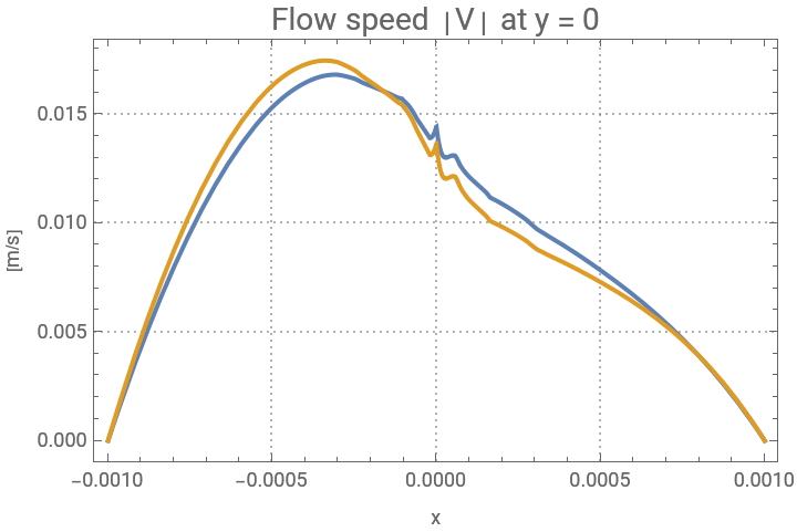
Plot+,+,x,-,,PlotTheme"Detailed",PlotLegends{"with correction","w/o correction"},PlotLabelStyle["Flow speed V at y = 0",14],FrameLabel{"x","[m/s]"},ImageSizeMedium
2
ufun[x,0]
2
vfun[x,0]
2
ufunCorrected[x,0]
2
vfunCorrected[x,0]
1
3
10
1
3
10
Out[]=
How the aforementioned model was obtained
How the aforementioned model was obtained
This section briefly presents how the model stated above was developed. First, an attempt was made to simply use the ElementMarker approach to indicate the region where each function should be applied.
Attempt #1: Using the If[ ElementMarker == 1, FluidFlowPDEComponent[...], BrinkmanPDEComponent[...] ] approach
Attempt #1: Using the If[ ElementMarker == 1, FluidFlowPDEComponent[...], BrinkmanPDEComponent[...] ] approach
This attempt explores using If[...] to combine the free-flow and porous media models. It highlights a parsing issue in Mathematica that needs to be resolved at the back end.
We note that when placing If[...] at the outer level, Mathematica does not parse the equations in the correct form. Instead, it treats the left-hand side of coupledFlowModel as a single element. Therefore, in the next attempt, we use Expand[...] to avoid placing If[...] at the outer level.
Attempt #2: Using Expand[...] to avoid placing If[...] at the outer level
Attempt #2: Using Expand[...] to avoid placing If[...] at the outer level
This attempt redefines the model by using Expand[...] to resolve parsing issues caused by placing If[...] at the outer level.
The coupled flow model appear to be solved, however the contour plot indicates a smaller-than-expected increase in velocity at the outlet. This suggests that the continuity equation is not being satisfied, possibly due to issues with the discretization of the PDEs.
To address this issue, one solution is to refine the mesh by lowering the MaxCellMeasure value. However, this approach may be memory-intensive.
It is worth noting that the continuity equation in the present model is formulated in a complex manner as shown below:
To address this issue, one solution is to refine the mesh by lowering the MaxCellMeasure value. However, this approach may be memory-intensive.
It is worth noting that the continuity equation in the present model is formulated in a complex manner as shown below:
The model is redefined with the reduced form of the continuity equation as follows:
These results match those from the example in [1], except for errors at the interface.
References
References
[1] COMSOL. “Forchheimer Flow.” Application Gallery, https://www.comsol.com/model/forchheimer-flow-4413. Accessed 11 July 2024.