ORIGINAL ARTICLE: Shen, Y., Zhang, Q., Shi, P. et al. Optical skyrmions and other topological quasiparticles of light. Nature Photonics 18, 15–25 (2024). https://doi.org/10.1038/s41566-023-01325-7
Article Abstract: Skyrmions are topologically stable quasiparticles that have been predicted and demonstrated in quantum fields, solid-state physics, and magnetic materials, but only recently observed in electromagnetic fields, triggering fast expanding research across different spectral ranges and applications. Here we review the recent advances in optical skyrmions within a unified framework. Starting from fundamental theories, including classification of skyrmionic states, we describe generation and topological control of different kinds of optical skyrmions in structured and time-dependent optical fields. We further highlight generalized classes of optical topological quasiparticles beyond skyrmions and outline the emerging applications, future trends, and open challenges. A complex vectorial field structure of optical quasiparticles with versatile topological characteristics emerges as an important feature in modern spin-optics, imaging and metrology, optical forces, structured light and topological and quantum technologies.
Introduction
Introduction
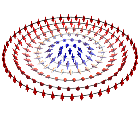
There usually are two ways to plot a skyrmion for visualizing its spin texture. The first one is to apply a color gradient onto the z-component of vectors. The z-colored representation can effectively reveal the particle confinement, but cannot reveal the structure of the transverse components (e.g., helicity and vorticity). To visualize the transverse-component distribution, another kind of color gradient map is used for the transverse azimuth. A full 3D vector components can be visualised using hue color to map the transverse azimuth from −π to π, and use changing brightness of the representation to map the z-component from −1 to 1, simultaneously.
The skyrmion vectors can be expressed as (Sx, Sy, Sz)=(Cos[ϕ+γ]Sin[θ], Sin[ϕ+γ]Sin[θ], Cos[θ]), and when γ=0, π, 2π the skyrmion is hedgehog-like and called Neel-type, when γ=π/2, 3π/2 the skyrmion is spiral-like and called Bloch-type. The following code can be used to illustrate the skyrmion in 3D and 2D, and by changing the parameter γ between 0 and 2π, a full evolution between Neel type, twisted type and Bloch type can be captured.
The skyrmion vectors can be expressed as (Sx, Sy, Sz)=(Cos[ϕ+γ]Sin[θ], Sin[ϕ+γ]Sin[θ], Cos[θ]), and when γ=0, π, 2π the skyrmion is hedgehog-like and called Neel-type, when γ=π/2, 3π/2 the skyrmion is spiral-like and called Bloch-type. The following code can be used to illustrate the skyrmion in 3D and 2D, and by changing the parameter γ between 0 and 2π, a full evolution between Neel type, twisted type and Bloch type can be captured.
3D skyrmion (in parameter space)
3D skyrmion (in parameter space)
Below are codes for representing three-dimensionally the skyrmion vectors in color gradient based on the z-component, Sz.
In[]:=
Clear["Global`*"]SetDirectory[NotebookDirectory[]];ColorData[1];Red1=RGBColor[1,0,0];Blue1=RGBColor[0,0,1];
Definition of the color scheme
new={{"Jet1","",{}},{"Gradients"},1,{0,1},{Blue,White,Red},""};AppendTo[DataPaclets`ColorDataDump`colorSchemes,new];AppendTo[DataPaclets`ColorDataDump`colorSchemeNames,new[[1,1]]];ColorData["Jet1"];mesh[θ_,n_]:=Table[{Cos[ϕ] Sin[θ],Sin[ϕ] Sin[θ],Cos[θ]},{ϕ,π/n,2 π,(2 π)/n}];p={{0,1},{π/6,12},{2π/6,15},{3π/6,19},{4π/6,15},{5π/6,12},{π,1}};points=Join[Flatten[mesh[#[[1]],#[[2]]]&/@p,1]];γ=π/2*4.0; (*Neel-type Skyrmion γ=0, Bloch-type Skyrmion γ=pi/2*)field[x_,y_,z_]:=Module[{θ,ϕ},ϕ=If[x^2+y^2>0,ArcTan[x,y]+γ,0];θ=ArcTan[z,Sqrt[x^2+y^2]];{Cos[ϕ]Sin[θ],Sin[ϕ]Sin[θ],Cos[θ]}]g1=VectorPlot3D[field[x,y,z],{x,-1,1},{y,-1,1},{z,-1,1},VectorPointspoints,VectorStyle"Arrow3D",VectorSizes0.6,VectorColorFunctionFunction[{x,y,z,vx,vy,vz,n},ColorData["Jet1"][vz]],AxesFalse];(*Plottheskyrmionvectorsin3Dspace*)R=0.94;g2=SphericalPlot3D[R,{θ,0,π},{Φ,0,2 π},ColorFunctionFunction[{x,y,z,θ,Φ,r},ColorData["Jet1"][z]],MeshFalse,BoxedFalse,AxesFalse,PlotStyleOpacity[0.22]];(*Plotthespherein3Dspace*)(*Belowplottheringsin3Dspace*)g3=ParametricPlot3D[{R Cos[u] Sin[π/6 1],R Sin[u] Sin[π/6 1],R Cos[π/6 1]},{u,0,2 π},BoxedFalse,AxesFalse,ColorFunctionFunction[{x,y,z,θ,Φ,r},Blend[{White,Black},5/6]],PlotStyleOpacity[0.7]];g4=ParametricPlot3D[{R Cos[u] Sin[π/6 2],R Sin[u] Sin[π/6 2],R Cos[π/6 2]},{u,0,2 π},BoxedFalse,AxesFalse,ColorFunctionFunction[{x,y,z,θ,Φ,r},Blend[{White,Black},4/6]],PlotStyleOpacity[0.7]];g5=ParametricPlot3D[{R Cos[u] Sin[π/6 3],R Sin[u] Sin[π/6 3],R Cos[π/6 3]},{u,0,2 π},BoxedFalse,AxesFalse,ColorFunctionFunction[{x,y,z,θ,Φ,r},Blend[{White,Black},3/6]],PlotStyleOpacity[0.7]];g6=ParametricPlot3D[{R Cos[u] Sin[π/6 4],R Sin[u] Sin[π/6 4],R Cos[π/6 4]},{u,0,2 π},BoxedFalse,AxesFalse,ColorFunctionFunction[{x,y,z,θ,Φ,r},Blend[{White,Black},3/11]],PlotStyleOpacity[0.6]];g7=ParametricPlot3D[{R Cos[u] Sin[π/6 5],R Sin[u] Sin[π/6 5],R Cos[π/6 5]},{u,0,2 π},BoxedFalse,AxesFalse,ColorFunctionFunction[{x,y,z,θ,Φ,r},Blend[{White,Black},2/11]],PlotStyleOpacity[0.6]];final=Show[{g1,g2,g3,g4,g5,g6,g7},BoxedFalse,ImageSizeMedium]
Out[]=

2D skyrmion (colored by z component)
2D skyrmion (colored by z component)
Below are codes for representing two-dimensionally the skyrmion vectors in color gradient based on the z-component, Sz.
In[]:=
size=0.035;(*theArrowsize*)coeff=0.07;(*Adjustthetubelengthofthearrow*)R1=0.;R2=1.;dtr=R2/6;(*numberofarrowlayers*)numarrow=Round[(r/dtr)*8];(*theArrownumbereverycircle*)x=rCos[phi];y=rSin[phi];z=0;theta1=π;(*Angleoftheskyrmioncentre*)theta2[r_]:=theta1-πr/R2;γ=+π/2*4.0;(*helicityπ/2Blochtype,πor0Neeltype,othersintermmediate*)(*allparametersareclarifiedabove*)mx1=coeff(Cos[phi+γ]Sin[theta1]);my1=coeff(Sin[phi+γ]Sin[theta1]);mz1=coeff(Cos[theta1]);mx2=coeff(Cos[phi+γ]Sin[theta2[r]]);my2=coeff(Sin[phi+γ]Sin[theta2[r]]);mz2=coeff(Cos[theta2[r]]);datain=FlattenTable{{x-mx1,y-my1,z-mz1},{x+mx1,y+my1,z+mz1}},{r,0,R1,dtr},phi,0,2π,,1;dataout=FlattenTable{{x-mx2,y-my2,z-mz2},{x+mx2,y+my2,z+mz2}},{r,R1,R2,dtr},phi,0,2π,,1;
2π
numarrow
2π
numarrow
The color is determined by mz
Neelin=Graphics3D[{ColorData["Jet1"][(Flatten[#][[6]]-Flatten[#][[3]])/2/coeff*0.5+0.5],Arrowheads[size],Arrow[Tube[#,size/4]]}&/@datain];Neelout=Graphics3D[{ColorData["Jet1"][(Flatten[#][[6]]-Flatten[#][[3]])/2/coeff*0.5+0.5],Arrowheads[size],Arrow[Tube[#,size/4]]}&/@dataout];Neel=Show[Neelin,Neelout];(*Belowplottheringsin2Dplane*)g1=ParametricPlot3D[{dtrCos[u],dtrSin[u],dtrCos[π/61]*0},{u,0,2π},BoxedFalse,AxesFalse,ColorFunctionFunction[{x,y,z,θ,Φ,r},Blend[{White,Black},dtr*1]],PlotStyleOpacity[0.8]];g2=ParametricPlot3D[{dtr*2Cos[u],dtr*2Sin[u],dtr*2Cos[π/61]*0},{u,0,2π},BoxedFalse,AxesFalse,ColorFunctionFunction[{x,y,z,θ,Φ,r},Blend[{White,Black},dtr*2]],PlotStyleOpacity[0.8]];g3=ParametricPlot3D[{dtr*3Cos[u],dtr*3Sin[u],dtr*3Cos[π/61]*0},{u,0,2π},BoxedFalse,AxesFalse,ColorFunctionFunction[{x,y,z,θ,Φ,r},Blend[{White,Black},dtr*3]],PlotStyleOpacity[0.8]];g4=ParametricPlot3D[{dtr*4Cos[u],dtr*4Sin[u],dtr*4Cos[π/61]*0},{u,0,2π},BoxedFalse,AxesFalse,ColorFunctionFunction[{x,y,z,θ,Φ,r},Blend[{White,Black},dtr*4]],PlotStyleOpacity[0.8]];g5=ParametricPlot3D[{dtr*5Cos[u],dtr*5Sin[u],dtr*5Cos[π/61]*0},{u,0,2π},BoxedFalse,AxesFalse,ColorFunctionFunction[{x,y,z,θ,Φ,r},Blend[{White,Black},dtr*5]],PlotStyleOpacity[0.8]];g6=ParametricPlot3D[{dtr*6Cos[u],dtr*6Sin[u],dtr*6Cos[π/61]*0},{u,0,2π},BoxedFalse,AxesFalse,ColorFunctionFunction[{x,y,z,θ,Φ,r},Blend[{White,Black},dtr*6]],PlotStyleOpacity[0.8]];final=Show[{Neel,g1,g2,g3,g4,g5,g6},BoxedFalse,ImageSizeMedium]
Out[]=
3D Hue colored skyrmion
3D Hue colored skyrmion
Below are codes for representing three-dimensionally the skyrmion vectors in hue color (for the transverse components, Sx and Sy) and brightness (for the z-component, Sz).
2D Hue colored skyrmion
2D Hue colored skyrmion
Below are codes for representing two-dimensionally the skyrmion vectors in hue color (for the transverse components, Sx and Sy) and brightness (for the z-component, Sz).
the color is determined by mx,my,mz at the same time: in detail, we use Hue function to characterize the Skyrmion. using the angle between mx and my to determine the priminary color, meanwhile using mz to determine the brightness and saturation of the whole figure in order to draw fancy Skyrmion picture
(********************************************************************************)
(********************************************************************************)
CITE THIS NOTEBOOK
CITE THIS NOTEBOOK
Topological quasiparticles of light: Optical skyrmions and beyond
by Yijie Shen
Wolfram Community, STAFF PICKS, May 30, 2022
https://community.wolfram.com/groups/-/m/t/2540813
by Yijie Shen
Wolfram Community, STAFF PICKS, May 30, 2022
https://community.wolfram.com/groups/-/m/t/2540813