Spiderwebs are highly optimized biological structures found in nature that exhibit high strength and resistance to damage, while being relatively material efficient. Understanding the mechanical behavior of these spiderwebs can provide insight into how the designs of elastic mesh structures can be optimized. This paper provides a two-dimensional linear elastic model for representing the stress patterns acting on an orb spider web with n and m number of radial and spiral threads respectively. This model is intended to provide a framework model for calculating optimal thread counts for an elastic net or web in the future. This model can be used in many areas of science, such as sea nets to collect garbage that need to stay intact for a long time. Additionally, this paper presents a two dimensional dynamic model composed of linear elastic threads that exhibit nonlinear behavior, consisting of n radial threads and m spiral threads, 4 enclosing frame threads, and four mooring threads. This dynamic model is used to estimate the time elapsed for a recently strummed spider web mesh to reach equilibrium. Following time, I analyze this dynamic model again, and show how linear elastic material modeling of individual threads can be used to model a non-linear elastic web by applying non-linear geometry. Future research should analyze how threads snapping affects affect the path to equilibrium and how a truly non-linear system of individual threads affects the model as a whole.
Introduction
Introduction
A spider web is a mesh made of a silk-like material crafted by spiders. Spiders use their webs in order to catch prey by coating their silk with various glycoproteins and salt, and reflecting ultraviolet (UV) waves that other insects get attracted to. Recent studies indicate that a spider web as a whole is non-linear elastic, but the threads themselves are linear elastic. A non-linear elastic system is one that returns to its original shape and size when a load is removed, but its resistance to deformation changes as it stretches or compresses. A linear elastic system is one that always bounces back to its original state, and where its stress is directly proportional to strain under Hooke’s law. In order to test linear elasticity in each thread, I will be applying tension to an orb web and analyzing how the web acts under two different models. I will measure elasticity with force measuring in my first model and in the second model time it takes to reach an equilibrium state, and see if these equilibrium states are different depending on the initial state.
Currently, research into spiders is a highly relevant field with many practical applications. For instance, when designing a fishing net that must be left out at sea for an extended period of time, manufacturers must take into account what pattern will be able to withstand the most damage and external interference. When addressing this problem, researchers look to spiders for their unique, naturally created, and structurally integral webs that stay hanging in adverse weather conditions and damage. Similarly, in space, such nets could be used to collect debris and clear up potentially harmful obstructions.
Initial Spider Web Setup
Initial Spider Web Setup
To begin work on the physics of my project I first needed to create a visualization of the spider web. For this purpose, I define the bulk of my global variables that I will be using throughout my project. To clarify, a radial thread will be defined as a line that goes from the center of my orb web and out to the edges. A spiral thread will be defined as a thread that does not connect to the center, is cyclic, and connects the acyclic radial threads.
Δ
α
Setting the number of spirals, number of radials, extra length extending past last spiral thread, angles, distance between each thread and width:
In[]:=
spiralNum=10;radNum=9;=(Pi/(radNum/2));radExtraLength=1;=1;widthMeters=5;graphicsWidth=N@(30*widthMeters/1000);
α
Δ
Spiral thread generation function using a parameterized function for a circle.
In[]:=
spiral[t_,r_]:={r*Cos[t],r*Sin[t]}
My original thought process was to use Partial Differential Equations that require a domain, so I started off with a region to represent threads in the spider web, rather than just 1D lines. As a minor note, this approach makes it easier to map colors representing force strength to my spider web in the future.
Using Wolfram’s built in Table step function, we can easily manipulate the step in order to get the geometry for the number of radial and spiral threads that we desire.
In[]:=
sp[length_,m_,thickness_,sides_] := Table RegionDifference Polygon[Table[spiral[t,k*length],{t,0,2Pi-Pi/(sides/2),Pi/(sides/2)}]], Polygon[Table[spiral[t,k*length-thickness],{t,0,2Pi-Pi/(sides/2),Pi/(sides/2)}]] ,{k,1,m};
Grabbing spiral coordinates and generating graphics of the spiral threads:
In[]:=
spiralCoords=Table[spiral[t,],{t,0,2Pi-,}];spirals=#&/@sp[,spiralNum,graphicsWidth,radNum]; Graphics[spirals]
Δ
α
α
Δ
Out[]=
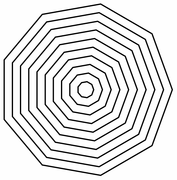
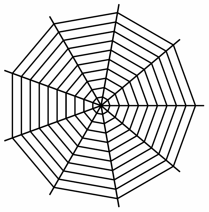
I generate radials with an extra distance going past the last spiral thread to allow for the visualization and calculation of the web being mounted on a tree or other object.
Generating radial threads by taking a rectangle with triangle tip and merging them together as a polygon:
In[]:=
genRads[m_,mSpace_,width_,radExtraLength_,sides_,discretize_]:=Module{x1,pEndTop,pMidEnd,pEndBot}, x1=((m*mSpace)-width)-(width/2)Tan[Pi/sides]+radExtraLength; pEndTop={x1,width/2}; pMidEnd={(m*mSpace)-width+radExtraLength,0}; pEndBot={x1,-width/2}; fullLength=m*mSpace+radExtraLength; rMeshRadThread=Ifdiscretize==False, {Polygon[{{0,-width/2},{0,width/2},pEndTop,pMidEnd,pEndBot}]}, Polygon[{{0,-width/2},{0,width/2},pEndTop,pMidEnd,pEndBot}]
Next, I needed to create any number of radial threads, and combine them into one full mesh primitive for future graphics. I did this by rotating each radial thread with in order to find the required angle to generate n number of radial threads that loop back to 0 degrees in n steps.
radNum*
π
radTotal
2
Generating all radial threads in a combined polygon:
In[]:=
genRadialPoly[m_,mSpace_,width_,radExtraLength_,sides_]:=MeshPrimitives[BoundaryDiscretizeRegion[RegionUnion@@Table[Rotate[genRads[m,mSpace,width,radExtraLength,sides,True],k*Pi/(sides/2),{0,0}],{k,0,sides}]],2]
Graphics generation of both radial and spiral threads:
In[]:=
radials=genRadialPoly[spiralNum,,graphicsWidth,radExtraLength,radNum];radLength=spiralNum*+(graphicsWidth/2)Tan[Pi/radNum]+radExtraLength*2;Graphics[{radials,spirals}]
Δ
Δ
Out[]=
As the physics in the paper I read relied on the intersection points of the spiral and radial threads, I had to find those points. While seeming trivial, slightly more goes into this than meets the eye, as we need to find the middle of each rectangular thread segment rather than the end or start of each one. I also define a function to grab the ends of each radial thread including extra radial length.
Generalized function to retrieve spiral and radial thread intersection points for future tension physics and graphics generation:
In[]:=
getSpiralIntersections[m_,mSpace_,width_,sides_]:=Table[{((m*mSpace)-width/2)Cos[k*Pi/(sides/2)],((m*mSpace)-width/2)Sin[k*Pi/(sides/2)]},{k,0,sides-1}];
Generalize function to retrieve radial thread endpoints:
In[]:=
getRadialEnds[m_,mSpace_,width_,radExtraLength_,sides_]:=Table[{((m*mSpace)-width+radExtraLength)Cos[k*Pi/(sides/2)],((m*mSpace)-width+radExtraLength)Sin[k*Pi/(sides/2)]},{k,0,sides-1}]
As I have many functions now, I decided to gather them all up with one spider web generation function. Now, a full spider web can be generated using just one call of the genSpiderWeb function.
Generalizing and grouping previous spiderweb generation functions :
In[]:=
genSpiderWeb[M_,mSpace_,threadWidth_,radExtraLength_,sides_]:=Module{spiralCoords,spirals,spiralLength,radials,radLength,intPts,endPts}, spirals=#&/@sp[mSpace,M,threadWidth,sides]; radials=genRadialPoly[M,mSpace,threadWidth,radExtraLength,sides]; radLength=M*mSpace+(threadWidth/2)Tan[Pi/sides]+radExtraLength*2; intPts=Table[getSpiralIntersections[t,mSpace,threadWidth,sides],{t,1,M}]; endPts=getRadialEnds[M,mSpace,threadWidth,radExtraLength,sides]; <|"Spirals"->spirals,"Radials"->radials,"RadLength"->radLength,"IntPoints"->intPts,"EndPoints"->endPts|>spiderWeb=genSpiderWeb[spiralNum,,graphicsWidth,radExtraLength,radNum];
Δ
As it would factor into my physics later on, I had to create a function in order to retrieve the length of spiral thread number . I did this by taking the Euclidean distance between each intersection point of the spiral thread. Then, tabling through this function, a list of the lengths of each spiral length can be achieved.
m
Function to find length of spiral thread number :
m
In[]:=
spiralLength[m_]:=If[m!=spiralNum+1,radNum*EuclideanDistance@@Take[spiderWeb["IntPoints"],m,2][[m]],radNum*EuclideanDistance@@Take[spiderWeb["IntPoints"],m-1,2][[m-1]]];spiralLengths=Table[spiralLength[t],{t,1,spiralNum}];
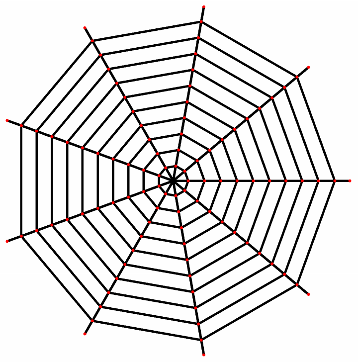
Here is a model of the base orb-weaver spiderweb. The red radial endpoints represent mounted connections with an external object, and red points in the web represent intersection points between spiral and radial threads.
Here is a model of the base orb-weaver spiderweb. The red radial endpoints represent mounted connections with an external object, and red points in the web represent intersection points between spiral and radial threads.
Graphics generation utilizing the new generalized spider web function:
In[]:=
Graphics[{spiderWeb["Spirals"],spiderWeb["Radials"],Red,Point[#]&/@spiderWeb["IntPoints"],Point[#]&/@spiderWeb["EndPoints"]}]
Out[]=
Generation of Tension Forces in Spider Webs Using Recursive Calculation
Generation of Tension Forces in Spider Webs Using Recursive Calculation
Here I move onto the physics of my project. In the paper a Simple Model for the Mechanics of Spider Webs (Aoyanagi, Y., & Okumura, K., 2010), the researchers discuss an orb spider web model, determining the tension at each intersection point of radial and spiral threads using a recursive equation. To start, I also had to find how much tension could be put on a thread before it breaks.
Determining the breakage force for a thread, radius, area, and spring constants:
Next I will derive a recursive matrix equation from the paper a Simple Model for the Mechanics of Spider Webs (Aoyanagi, Y., & Okumura, K., 2010):
M reliant variables for my recursive equation:
Calculating force at spiral m utilizing spiral spring constant k. I also derive lists to store the color on the rainbow that would correspond to the current tension force magnitude acting on a node for any given moment in time for the spiral and radial threads:
Taking the spiral points in a list:
As a simple test, we can see if a radial thread in the spider web has broken by comparing all the forces on all the intersection nodes and seeing if that force exceeds the breakage force of the spider thread.
Finding if a radial thread has been broken:
Next, I map the colors derived from my forces onto my radial threads using blend, polygon, and mesh properties.
Mapping the colors I generated dependent on force magnitudes onto my spider web mesh:
Next, I wanted to test the force equations with different spiral spring constants in order to simulate general damage to the spider web.
simDamage function that can generate a spider web with forces applied at each node, and table through my graphics generation of the web eight times in order to increase the spring constant:
Running the simDamage function in order to simulate damage to a spider web slowly taking more and more damage by increasing the general spring constant k. This simulates if a spiral thread or two broke and the reliance on spiral threads increases.
Next I wanted to test different amounts of radial and spiral threads under ideal conditions in order to simulate how different kinds of spider webs have unique tension patterns:
In order to simulate how tension distributes across spiderwebs with different amounts of radial and spiral threads, I start from a triangular web with a number of radial threads greater than or equal to 3, and a number of spiral threads greater than or equal to 1:
As observed above, with an increase in radial threads and spider threads come with an increase in overall tension, but it is only marginal over small increases. For example, the range of overall tension max increase is minimal in a 10 spiral, 10 radial thread model compared to a 5 spiral, 5 radial thread model. An interesting observation from these models is that the highest tension in the spiral threads is concentrated in the center of the spiral webs, contrary to my original thinking that it would be the outermost threads.
Finally, I wanted to test wether the elasticity in my models was linear or nonlinear as one goes from the center of the spider web to the outskirts.
Setting up bar charts for forces applied at each node in my spiderweb model:
After studying the Japanese research paper and analyzing the stress patterns in spider webs, I have realized multiple limitations with their model. One to be that the model only calculates the magnitude of the forces at each node instead of direction vectors, so it is impossible to derive movement from the model in order to show a linear or non-linear elastic system. Second, is that the model is very strict to a basic orb pattern, and the force becomes almost completely independent of the number of radial threads, other than the radial spring constant. This causes the model to become fully linear elastic, and somewhat unrealistic of how a real spider web acts. For these reasons, I have decided to move onto an Ordinary Differential Equation (ODE) model of spider webs in order to better model the tension in the spiderweb and dynamically simulate the movement of the spiderweb from rest when tension is applied.
Moving to an ODE System
Moving to an ODE System
For my ODE system to model the movement of a spider web, I decided I wanted to create a more realistic orb web. This can be done by generating an inner spider web that connects to an outer square thread perimeter, and finally four fixed mooring threads with the edge points fixed. In addition, I will be assuming that the web is vertical in order to simplify the model to 2D space. Lastly, any thread specific biological values have been derived from a 2012 paper (Cranford, S. W., Tarakanova, A., Pugno, N. M., & Buehler, M. J.) in their study of spider webs. Again, I will be using linear elasticity for each individual thread, and analyzing the resulting model of the spider web as a whole.
Here I will begin by defining global variables that I will be using over the course of my simulation. This includes the thread diameters, Young’s modulus, breaking stress, and initial tension for each kind of thread in the model.
Pressure at which thread snaps:
Young’s modulus of elasticity for each thread:
Width of individual threads:
Initial tension of threads:
Here I redefine other variables that I will be using over the course of my ODE model.
First, I define Ns and M as the number of radial and spiral threads respectively, mass is the total mass of a generic spider web in kg, and totalNodes is the number of nodes in the spider web (center+radials+spirals+rect vertices+mooring points):
Calculating the above formula with a function:
Getting the square vertex points of the frame:
Getting the mooring points:
Here I define the variables that will hold the positions of my square vertices, radial, spiral, and mooring points. In addition, I define the initial resting position of each point. In my code, an i stands for the current radial thread, and a j stands for the current spiral thread. The center will be defined as i = 1, j = 0, so as to simplify the code. Radial threads start at i = 1 from angle zero, and loop around counterclockwise. Spiral threads start at j = 1 (excluding the center), and increase as you go out.
Spiral and radial point definitions combined in one through points:
Mooring joint (fixed) and resting position joint definitions:
Defining the functions that will allow for the calculation of finding which radial threads are closest to each square vertex. This depends on the angle separation of each radial thread, making the calculation somewhat difficult. The calculation is to take the floor of the number of radial threads, multiplied by the angle of whichever square vertex one is trying to find the points closest to, and finally taking the radial total number mod of this number and applying a displacement of 1 to account starting from radial thread 1 instead of 0. This process find the nearest radial thread clockwise to the vertex, and a similar process, but taking the ceiling of the number of radial threads can be applied to find the nearest radial thread counterclockwise.
Determining points close to frame vertices:
Now I define the functions for determining neighboring nodes to spiral and radial joints. In Mechanics in Naturally Compliant Structures, a grid system is introduced for calculating this, with 4 connection points to each node, the upper node is defined to be s = 1, left s = 2, bottom s = 3, and right to be s = 4. I propose a spiral system to calculate this instead. In this system, I represent a change counterclockwise or clockwise with s = 1 or 2 respectively. In addition, I represent a change to an inner radial thread or outer radial thread with s = 3 or 4 respectively. This needs to be done twice, once for the points with respect to time, and once for the points at rest in order to get an accurate model that can be solved in Wolfram.
Finding neighbor spiral and radial thread joints to a specified joint[i,j]:
Finding neighbor resting spiral and radial thread joints to a specified restingJoint[i,j]:
Below I define a similar method of finding the closest points to my rectangular frame vertices using my previously defined functions isCloseRectPoint and findNearestPoint. The system works the same, with s = 1 and s = 2 being the point counterclockwise and clockwise to the vertex respectively. Similarly, a resting function for this is also needed in order to accurately simulate this system in wolfram.
Finding neighbor frame joints to a specified frame vertex joint:
Finding neighbor resting frame joints to a specified frame vertex joint:
Calculating radius’ of each thread type:
Calculating spring constants for each thread type:
Force calculations for each thread type:
Initialization code for the joints I will be using for my spiderweb simulation. Although it looks like the definitions stay undefined, they get temporary assignments when ran through NDSolve - the function to solve systems of ODEs:
Initial conditions for the ODE system. This function takes in three parameters: spiral amount, radial amount, and a random distance factor to each node. It is the random distance factor that I am applying to each node which simulates a web that has recently been hit or strum. I define the initial position for all of my joints in the spider web, and then go on to define all of the starting velocities to have zero direction (assuming no external force other than tension is being applied).
Setting initial positions of joints to predetermined joint geometry and setting velocities to zero:
Defining the different dampening constants used in my system for each thread:
Defining the ODE system of equations to evaluate spider web joint positions at time t:
A simple function telling NDSolve how many dependent variables to solve for:
Grabbing the resource function for finding interpolating function’s domains in order for use in my NDSolve:
Defining an update geometry function in order to dynamically update the geometry of each joint in my spider web:
Here I set the parameters of my ODE system such as radial and spiral amount, frame size, spiral spacing ratio, and randomness of spiderweb nodes:
Here I set the elasticity and initial tensions in my system
Creating one clean function in order to represent my web dynamically with the press of a button. In order to use this dynamic module, the reader must download the notebook and open it in Wolfram desktop. Note: A limitation of this current model is that threads can not break. If any weird geometry is seen other than at the start, that is usually a sign a thread has been broken.
Dynamic module that generates a spider web moving to a force equilibrium from user inputted and randomized starting joint positions. Although this does not work in cloud, for now it is still needed to run my simulation below:
Running my system of ODEs with ND Solve, then partitioning in order to grab interpolating functions as coordinate pairs:
Now, I had to generate nodes for graphical use, grabbing interpolating functions as coordinate pairs.
Partitions points into radial sets:
Turns radial sets into spiral coordinate order:
Converts nodes to an easily manipulable form:
Finds two closest radial lines to frame vertex i, for i from 1 to 4:
Creates quad connections between vertices close to square frame:
Gets center node:
Gets all coordinate pairs in some radial thread:
Gets all coordinate pairs in some spiral thread:
Gets coordinate pairs of the frame:
Gets coordinates of mooring threads:
Now, I wanted to generate graphic output to demonstrate my web simulation.
Creates Manipulate to visualize web over time:
Running the previous system with original tensions:
Running the previous system with doubled tensions:
Defining lists containing values of just the radial = 1, spiral = 1 joint over an approximately smooth timespan:
Finding displacement values for each system:
Creating a plot of the radial = 1, spiral = 1 joint over time for the original initial tension and doubled initial tension systems:
From this graph I was able to conclude two things: the path to equilibrium is not linear, and the final displacement for each system is not proportional to one another even when proportional initial tension values. In a purely linear elastic model of a spider web, changing the initial tension would scale the internal forces proportionally and end up scaling displacement proportionally in turn. As my model contradicts this - the displacements are not proportional - I have showed that changed in initial tension affect the final equilibrium and displacement in my model. Hence, I have successfully demonstrated non-linearity using linear elastic Hookean based individual threads.
Conclusions
Conclusions
Over the course of this project I have developed realistic simulations of how tension distributes throughout a spiderweb using recursive matrix algorithms, and modeled spider web movement from a randomized position in order to simulate damaged or strummed webs under tension. Contrary to my original thinking, I have found that even with treating each individual thread as linear elastic, due to a spiderwebs complex and interconnected properties, the spider web reaches an equilibrium in a different state for every randomized run, rather than returning to one set state for all runs. This, and my final graphs showing displacement between varying initial conditions, accomplishes the goal that I set in my introduction to test if non-linear elastic modeling of a spider web can be accomplished with individual thread linear elastic modeling. In addition, I was able to accurately model down to the millisecond how long it takes for a strummed spider web to reach equilibrium under tension, taking into factor different spider thread material properties. These findings will be useful in the modeling of hyperelastic spider and net simulations in order to optimize mesh based tension.
Future Directions
Future Directions
I am currently working on a simulation that allows for the web to start with n number of threads cut. In addition, I will incorporate into this model the ability to dynamically delete broken threads from the graphic and have the web either completely break or reach equilibrium again dependent on the solutions of the ODE system. This would help with long term damage modelling and optimizations for net patterns that need to meet market standards for durability. After this, I would hope to model my web in 3D, and try to create physical replications of my webs, or even do randomized mesh’s in order to find the strongest elastic patterns possible.
References
References
◼
Alam, M. S., Wahab, M. A., & Jenkins, C. H. (2007). Mechanics in naturally compliant structures. Mechanics of Materials, 39(2), 145–160. https://doi.org/10.1016/j.mechmat.2006.04.005
◼
Aoyanagi, Y., & Okumura, K. (2009). Crack-Tip Stress Concentration and Structure Size in Nonlinear Structured Materials. Journal of the Physical Society of Japan, 78(3), 034402. https://doi.org/10.1143/jpsj.78.034402
◼
Aoyanagi, Y., & Okumura, K. (2010). Simple Model for the Mechanics of Spider Webs. https://doi.org/10.1103/PhysRevLett.104.038102
◼
Cranford, S. W., Tarakanova, A., Pugno, N. M., & Buehler, M. J. (2012). Nonlinear material behaviour of spider silk yields robust webs. Nature, 482(7383), 72–76. https://doi.org/10.1038/nature10739
◼
Regassa, Y., Lemu, H. G., Sirabizuh, B., & Rahimeto, S. (2021). Studies on the Geometrical Design of Spider Webs for Reinforced Composite Structures. Journal of Composites Science, 5(2), 57. https://doi.org/10.3390/jcs5020057
Acknowledgements
Acknowledgements
To begin, this project would not have been possible without my mentor, Angel Rojas, for supporting me throughout this program. From being my advocate, to mentor, to giving me confidence when I was at a crossroads on project decisions, and providing guidance for my project. I would also like to thank Shenghui for lending a helping hand when I was confused with how to work out the new ODE physics for my project. Along with the above, I have to thank the rest of my mentor group, dorm mates, Qianheng Xu, Arnay Garhyan, TAs, mentors, and wolfram program directors Rory Foulger, Eryn Gillam, and Megan Davis. Last but not least, I want to express my gratitude to Stephen Wolfram for making this program and project possible.
CITE THIS NOTEBOOK
CITE THIS NOTEBOOK
Dynamic modeling of a 2D spiderweb's elastic behavior
by Jonah Caplan
Wolfram Community, STAFF PICKS, July 9, 2026
https://community.wolfram.com/groups/-/m/t/3754178
by Jonah Caplan
Wolfram Community, STAFF PICKS, July 9, 2026
https://community.wolfram.com/groups/-/m/t/3754178