We offer a computational model for evaluating tradeoffs between life and progress. Our framework evaluates people as cells in a one-dimensional outer-totalistic cellular automaton with two living states and an absorbing output state of death. Pandemics are modelled as instant death for a portion of the population and government regulations are modelled as lockdown restrictions on the number of consecutive neighboring cells in a certain state. With this model, we are able to compare the implicit trade-off between an unchecked yet instant pandemic and a continual governmental lockdown. We find that lockdowns lead to reduced complexity and increased death compared to a pandemic. If people are allowed to vote, they tend to vote for lockdowns early but regret their choice later. The findings suggest generally that societies can be robust to external attacks but can wither from internal attempts to control the mechanisms of progress.
1. Introduction
1. Introduction
There are two fundamentally different ways of modeling phenomenon: from the top down and from the bottom up.
Top-down approaches start with stylized facts and calibrate models with continuous parameters to match those stylized facts as closely as possible. Bottom-up approaches first aim to simplify the problem as much as possible and then explore the resulting computational universe.
Top-down approaches are the contemporary dominant standard in the scientific literature, even to the extent of how papers are structured, with claims outlined first, then a method, results, and discussion. However, per Wolfram (2002)'s Principle of Computational Irreducibility, a bottom-up approach can never in principle be expressed in such a way, because it would be impossible to know ahead of time the results of an arbitrary computation. Therefore, this paper is organized in a way that may appear less conventional but is more appropriate to the computational exploration approach.
Section 2 argues for, models, and finds the unique minimal computational model of society. Section 3 applies that model to a world where a pandemic can instantly kill some of the participants, or a lockdown can prohibit certain kinds of social interactions. Section 4 concludes with suggestions for future research.
2. The Minimal Model of Society
2. The Minimal Model of Society
We model the state of society as a cyclical list of people. Each person can be in one of three states: happy, sad, or dead. Death is an absorbing state. These states can also be interpreted in the standard SIR model as healthy/susceptible, infected, and dead.
Color the three states as happy black, sad white, dead red, with a mesh border on cells only for short examples by default:
In[]:=
SocietyPlot[states_,mesh_:Automatic]:=ArrayPlot[states,MeshReplace[mesh,AutomaticLength@Flatten@states<100],ColorRules{0Red,1White,2Black}]
Example state of two happy people, one sad person, and one dead person:
SocietyPlot[{{2,2,1,0}}]
Out[]=
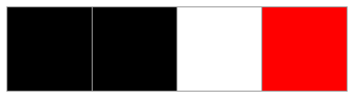
Each person transitions to a new state depending on their own current state and the states of their nearest living neighbors. Dead neighbors are ignored.
Ignoring dead neighbors effectively shrinks a society, but we keep the strands of red to be able to visualize death over time.
People care about how their living neighbors are doing, whether they are happy or sad, but they only care about the total. It doesn't matter if it's your left-neighbor who is sad and your right-neighbor who is happy or vice versa. This is commonly referred to as an “outer-totalistic” rule.
However, it is not a standard outer totalistic rule because there are two input colors but three output colors: a dead person does not evolve, but a living person can be either sad or happy and can become either sad, happy, or dead.
How many distinct initial states are there for each person, assuming a neighborhood region or radius of r? Temporarily renumber the states as zero for sad and one for happy in order to count the number of possible totals. Then the person evolving can be in one of two states, and the total of his 2r neighbors can be anywhere from zero to 2r, which is 2r + 1 possibilities. That's 2 · (2r + 1) possible initial states for each person.
How many different rules are there? Each of those possible initial states can be mapped onto one of three outputs, so there are 3 to the power of 2 · (2r + 1) possible rules.
Function for the maximum number of possible rules for a given neighborhood radius:
In[]:=
MaxRules[r_]:=3^(2(2r+1))
Compute the number of possible rules for regions up to five neighbors on either side:
AssociationMap[MaxRules,Range@5]
Out[]=
1729,259049,34782969,4387420489,531381059609
Thus, there are 729 one-neighbor outer-totalistic rules from two-color inputs to three-color outputs.
Define a function to evolve the center cell of a list of cells of length 2r +1:
In[]:=
me[rule_][cells_,r_]:=With[{mid=cells〚r+1〛},IntegerDigits[rule-1,3,2(2r+1)]〚2rmid+Total[cells]+1〛]
For a neighborhood radius of one, the function defined above takes a rule number from 1 to 729 and returns a function that takes a list of three black or white cells and the number 1 to evolve the center cell to either white, black, or red.
For example, according to rule 92, a sad person surrounded by one happy neighbor and one sad neighbor will evolve to be happy in the next step, regardless of which neighbor is which.
Example evolution from an initial state of {happy, sad, happy} for rule 118:
{me[92][{0,0,1},1],me[92][{1,0,0},1]}
Out[]=
{1,1}
Display the rule plot for a given rule:
In[]:=
SocietyRulePlot[rule_,r_]:=Table[Show[SocietyPlot[{1+input,{None,1+me[rule][input,1],None}}],ImageSize75],{input,Tuples[{0,1},3]}]
Row[SocietyRulePlot[92,1],Spacer@2]
Out[]=

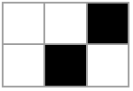
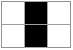
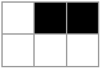
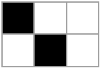
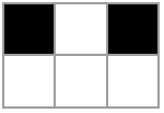
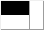
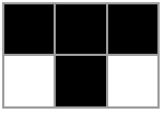
In fact, rule 92 always results in a happy black cell if all three cells are happy or if exactly one of the three is happy and the others sad. If nobody is happy, or two people are happy and one is left out, then the cell becomes sad.
To evolve the state of an entire society for one step, we can use our custom evolution rule in the specification of a cellular automaton if we first delete all dead cells and remap sad and happy to zero and one, and then map the output colors back to one, two, and three, where color three is then mapped back to state zero in our original numbering system to indicate a dead cell, and reinsert those new values in the original state to maintain the positions of the unevolving dead cells.
Function to evolve society for one step for a given rule, radius, and initial condition:
In[]:=
EvolveSocietyOneStep[rule_,r_,in_:{0|1|2..}]:=Module[{t=in,p=Flatten@Position[in,1|2]},t〚p〛=1+Last@CellularAutomaton[{me[rule],{},r},DeleteCases[in,0]-1,1];t/.(30)]
For example, we can evolve our initial condition above.
Evolve rule 92 on a radius 1 of the initial condition happy, happy, sad, dead:
SocietyPlot[List@EvolveSocietyOneStep[92,1,{2,2,1,0}]]
Out[]=
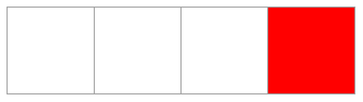
Everyone who was happy becomes sad, the sad person stays sad, and dead people remain dead.
Note that our initial conditions for the present analysis will always be a fixed number of people, rather than a constantly growing population. Therefore, every rule will eventually cycle, some faster than others. To evolve society for multiple steps, we simply repeat the process, stopping early if we ever find ourselves in a cycle.
Function evolve society up to a maximum number of steps, stopping early if a cycle is detected:
In[]:=
EvolveSociety[rule_,r_,in_:{0|1|2..},t_,onestep_:EvolveSocietyOneStep]:=NestWhileList[If[Length@DeleteCases[#,0]<2r+1,ConstantArray[0,Length@#],onestep[rule,r,#]]&,in,DuplicateFreeQ[{##}]&,All,t]
For example, evolve rule 92 for ten steps on the same initial condition:
SocietyPlot[EvolveSociety[92,1,{2,2,1,0},10]]
Out[]=
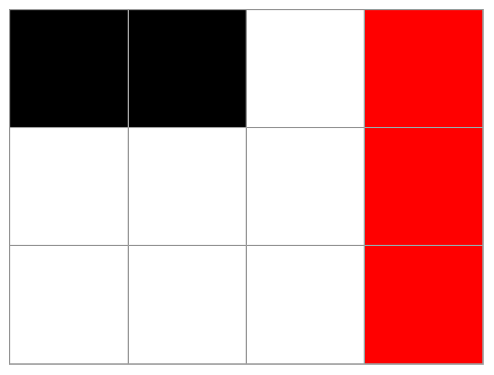
Notice that for the given initial condition, rule 92 cycled after two steps, so it did not evolve all ten required steps. From step 2 to step 3, the evolution does nothing, so all future steps would look the same: three sad people and one dead one.
We typically wish to filter out cyclical evolutions and explore the space of possible evolutions, ignoring simple equivalencies such as rules that are identical except the identification of sad and happy.
Given a radius, initial state, max number of time steps, evolve either a random sample or all possible inequivalent max-length rules:
In[]:=
EvolveAllSocieties[r_,init_,t_,n_:All]:=DeleteDuplicatesBy[MaximalBy[AssociationMap[EvolveSociety[#,r,init,t]&,If[n===All,Range[MaxRules@r],If[ListQ@n,n,RandomInteger[{1,MaxRules@r},n]]]],Length],With[{c=Counts@Flatten@#},If[Lookup[c,1,0]>Lookup[c,2,0],#,#/.{21,12}]]&]
Starting with a standard initial condition of one happy person in the middle of one hundred sad people, we can explore all of the possible 729 rules for emergent complexity. While we define complexity more specifically below, for now without loss of generality we select only those evolutions that have the maximal length before they cycle.
Standard initial condition:
SocietyPlot[List[startStandard=Join[ConstantArray[1,50],{2},ConstantArray[1,50]]]]
Out[]=

Plot labeled evolutions with a potentially uneven number of plots in a grid-like format:
In[]:=
LabeledGraphicsGrid[a_,max_:8,img_:600]:=GraphicsColumn[GraphicsRow/@Partition[Show[#2,PlotLabel#1]&@@@Normal[a],UpTo@max],ImageSizeimg]
Plot all maximally complex radius-1 rules for the standard initial condition and 500 time steps:
LabeledGraphicsGrid[SocietyPlot/@EvolveAllSocieties[1,startStandard,500]]
Out[]=
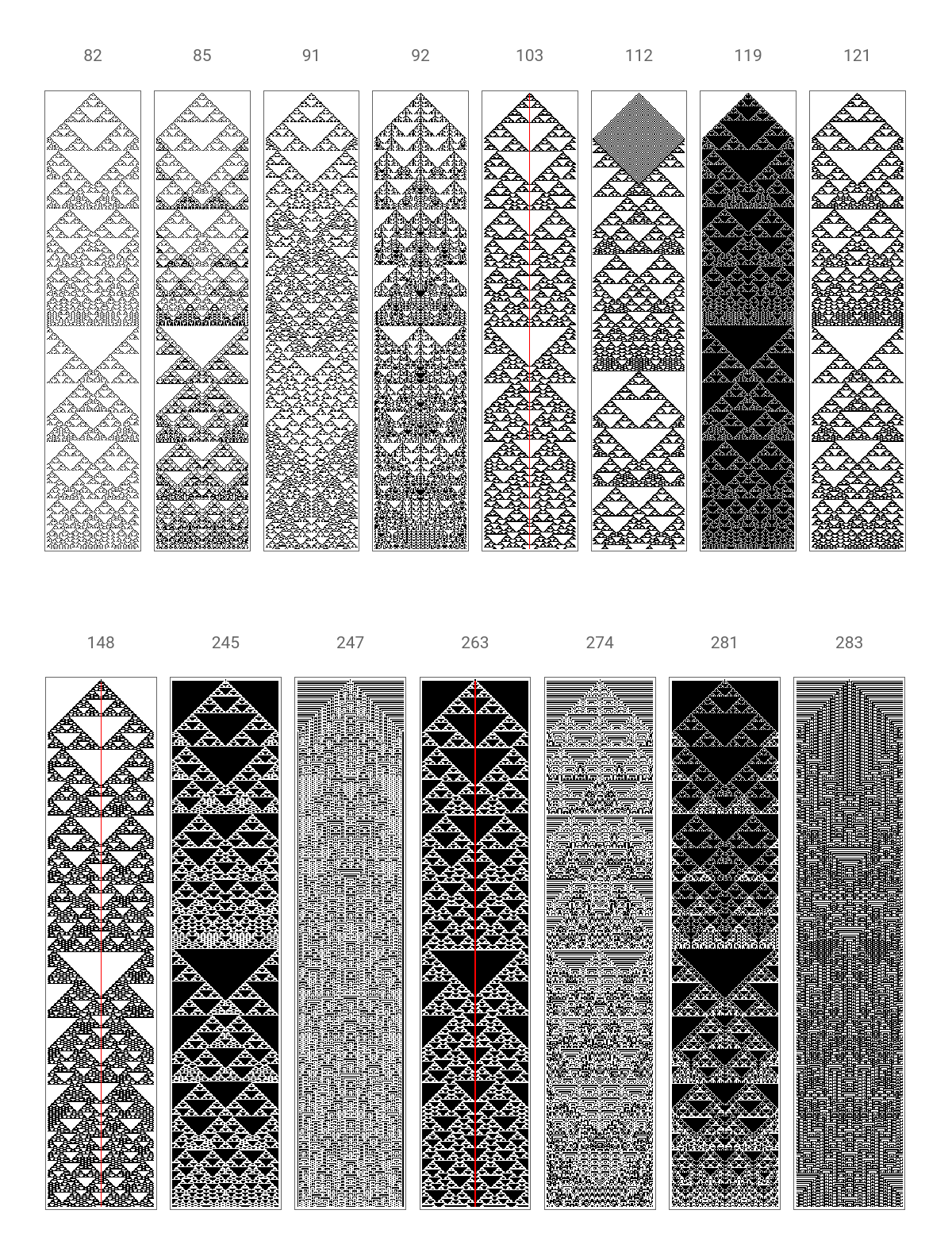
There is some interesting structure but the evolution is mainly symmetric. Rules 103, 148, and 263 are somewhat amusing as the first happy person dies immediately, and that is the only death.
What if we start with an asymmetric initial condition?
Define an asymmetric starting condition of one sad, two happy, three sad, and so on, for a total length of 91 cells.
Evolve all societies for 500 time steps from the asymmetric start condition:
These evolutions appear far more interesting and complex. Compare these to the evolutions starting from a random initial state with the same number of people.
Evolve all societies for 500 time steps from a random initial condition of the same length:
Most of the complex rules are common across both initial conditions, suggesting both that our asymmetric initial condition might be sufficient for evaluating the rules, and that the rules themselves exhibit a consistency in terms of complexity.
Compute the length of the both evolutions and their intersection:
Complexity can be measured in one of two ways. The complexity pictured above was a time-series complexity: given a rule, evolve the society, and evaluate the complexity of the resulting evolution. An alternative measure of complexity is cross-sectional complexity: for each possible rule, evolve all possible initial conditions by one step, and count how many distinct output states they have, and rank the rules by that number. This measures how complex a rule is relative to other rules.
We can then filter for rules that are consistently complex by recursively filtering for rules with the maximal cross-sectional complexity for increasingly large population sizes. That would indicate that the rules we find are not only complex for a given population level, but tend to be complex for various population levels; thus, they are intrinsically complex.
Starting with a population of 5, evolve every rule one time step from each of 1000 different random starting conditions, and keep the rules with maximal distinct outputs. Recursively filter further on doubling population sizes 5, 10, 20, 40, 80:
Of the 729 possible rules, 144 are consistently cross-sectionally complex. Let's evolve them on our asymmetric starting condition and see what they look like, transposed because of their thinness for better visibility.
Evolve all of the 144 consistently cross-sectional complex rules for 1000 time steps, and display the evolution left-to-right:
Only two maximally complex rules remain: 92 and 274. Note that this is a subset of all the maximally complex rules for 1000 time steps only, because we pre-filtered only for those rules that maintain their characteristic complexity across a variety of population amounts.
Compute the rule numbers of the maximally complex rules for 1000 time steps only:
We examined the rule plot for rule 92 above. We can compare rules 92 and 274 side-by-side to see if they have any common patterns.
Display the rule plots for rules 92 and 274:
By inspection we can see that rule 92 is the exact opposite of rule 274: whenever rule 92 would evolve to a black cell, rule 274 evolves to a white cell, and vice versa.
Therefore we can without loss of generality call rule 92 the unique minimal model of society.
3. Pandemic vs. Lockdown
3. Pandemic vs. Lockdown
One way to implement the effect of an unchecked pandemic is to presume that some portion of the population will die immediately. This effectively assumes that some portion of the population would remain alive after a pandemic, even without lockdowns, quarantines, social distancing, or any other changes. Equivalently, some portion of the population is deemed immune.
Suppose for concreteness the first n columns all die instantly from an unchecked pandemic; an unchecked pandemic is one that is not in any way mitigated by social distancing, masks, vaccines, lockdowns, quarantines, or any other changes in human behavior. What would the remaining evolution of rule 92, the minimal model of society, look like?
Let's consider a random initial condition and suppose one quarter of the population would be instantly killed. We evolve 2,000 time steps.
Set a fixed random initial condition:
Evolve both the original and the pandemic societies for 2000 time steps:
In this case, an instant 25 percent death rate does not thwart the remaining complexity and it does not cause any further deaths.
As an alternative, consider a government intervention criminalizing happy associations above a certain threshold. For example, suppose government edicts make any sequence of ten or more happy black cells illegal. Since any government law can ultimately be enforced only by violence, for a minimal model interpretation we can implement such a policy as instantly killing any sequence of three or more black cells, i.e., by converting their state to red.
Define a function to kill k or more consecutive black cells:
Show how it works on the asymmetric initial condition for k = 10:
Define a one-step society evolution in the presence of such a ten-person lockdown:
Evolve the original, pandemic, and lockdown societies for 2000 time steps:
In a lockdown, for both rules, fewer people die initially, but ultimately result in a total annihilation of the entire population, making the pandemic's instant but one-time population reduction of 25 percent seem utopian by comparison.
What if we allow voting? Suppose each column in the evolution is a single person who can vote either for or against government-enforced lockdowns. However, each person is cognitively or computationally limited and can only forecast their own state one row into the future. In other words, at the time of the vote, each person looks at his or her neighbors and forecasts their own cell color in the next time step. They then vote for the program that makes them happy, or at least sad but alive. In the event of a tie, they abstain.
Consider such a vote at the initial time above. The first 25 people who would be instantly killed by an unchecked pandemic would surely all vote for the lockdown, because sad or happy is better than dead. Of the remaining 75 people, one person (ironically, the 26th, the first one not to die from the instant pandemic, who would be sadder under a lockdown) would vote for the unchecked pandemic, and one person would vote for the lockdown (the last one not to die from the instant pandemic, who would be happier under a lockdown). Thus the vote would be 1-26 in favor of the lockdown, with 73 abstentions.
Define a function to display the evolution of an unchecked pandemic vs. a lockdown after a given number of time steps:
Evaluate the vote based on the first time step of the evolution:
We can evaluate how the instantaneous vote would look across time. Initially, and for the first few time steps, votes are overwhelmingly in favor of lockdown. Then it becomes contentious until about the 50th time step, after which the majority of living voters would have consistently preferred the pandemic.
Plot the vote tallies for lockdown vs. pandemic across time:
4. Conclusion
4. Conclusion
Our model has effectively no parameters. It has not been calibrated to actual parameters of the Covid-19 virus. Lockdowns and other government measures aimed at reducing the spread of the pandemic are far more complicated than merely murdering adjacent happy neighbors. Most devastatingly of all, our society surely is not a one-dimensional outer-totalistic cellular automaton operating on a fixed population.
Instead, the aim of this model was to generate with the simplest possible mechanism the possible effects of government intervention vs. non-intervention. With a simplest-model approach, the goal is not to provide immediately actionable policy implications but rather to explore, illustrate, and compare counterfactual scenarios in a deterministic but computationally irreducible model.
Future extensions can explore higher radii, incorporating randomness or time delays in pandemic deaths or government regulations, allowing for changes in the evolutionary rules, and extending the voting forecast window.
As a general explanation, these illustrations and explorations suggest that a society can be automatically robust to an external attack such as a pandemic but that attempts to tweak the evolution in the name of safety may in fact make the society more fragile overall. Such government interventions will at first have widespread support but eventually people will have regretted allowing the government interventions in the first place.
References
References
◼
Maymin, Philip Z. (2009), “Regulation Simulation”, European Journal of Finance and Banking Research 2:2, 1-12.
◼
Maymin, Philip Z. (2011), "The Minimal Model of Financial Complexity," Quantitative Finance 11:9, 1371-1378.
◼
Maymin, Philip Z. (2013), “A New Kind of Finance,” in Irreducibility and Computational Equivalence: 10 Years After Wolfram’s A New Kind of Science, Hector Zenil, ed., Springer Verlag.
◼
Maymin, Philip Z. (2014), “A New Algorithmic Approach to Entangled Political Economy: Insights from the Simplest Models of Complexity,” in Steven Horwitz, Roger Koppl (ed.), Entangled Political Economy (Advances in Austrian Economics, Volume 18), Emerald Group Publishing Limited, 213-236.
◼
Weisstein, Eric W. "SIR Model." From MathWorld--A Wolfram Web Resource. https://mathworld.wolfram.com/SIRModel.html
◼
Wolfram, Stephen (2002). A New Kind of Science. Wolfram Media. https://wolframscience.com