I use the powerful built-in functions: Probability, ProbabilityDistribution, DiscreteMarkovProcess and so on, to understand the details of the classic probability problem about Markov process, networks and finally relate to the famous Sierpinski triangle.
Problem
Problem
Given 6 healthy seeds on day 0, the probability of a seed growing into flower is 50% on any given day N (N= 1,2,3,4 ...) and we assume the flower never dies.
Question: What is the average (expectation) days we shall wait to see six flowers for the first time starting from day 0?
Question: What is the average (expectation) days we shall wait to see six flowers for the first time starting from day 0?
Analysis
Analysis
Assume the probability of success/flowering on each day is and we see 6 flowers for the first time after waiting days. I use the built-in symbolic function to directly model the process:
p
n.
In[]:=
With{p=1/2},expr=SimplifyProbabilityMax[a1,a2,a3,a4,a5,a6]==n.-1,{a1GeometricDistribution[p],a2GeometricDistribution[p],a3GeometricDistribution[p],a4GeometricDistribution[p],a5GeometricDistribution[p],a6GeometricDistribution[p]},Assumptions->n.∈PositiveIntegers
Out[]=
-6n.
2
1+n.
2
2+3n.
2
1+5n.
2
n.
4
n.
16
The code above is simple. For instance we see 6 flowers for the first time on day 6. This means the last seed or seeds grow into flower exactly on day 6, which is the largest value across the lifetime of all six seeds. Here the Max function works just as expected for this property.
Verify the expression for the first day:
In[]:=
expr/.n.->1
Out[]=
1
64
Compute the average using the definition of expectation:
In[]:=
res1=Sumn.*expr,n.,1,Infinity
Out[]=
7880
1953
On average We need to wait about 4 days to see 6 flowers:
In[]:=
res1//N
Out[]=
4.03482
Or use customized to create a distribution function and then use function to compute the expectation:
In[]:=
=ProbabilityDistribution"PDF",(-63+93+35+3-225-45),n.,1,Infinity,1;
-6n.
2
1+n.
2
2+3n.
2
1+5n.
2
n.
4
n.
16
In[]:=
Simplify[CDF[,t],Assumptions->t∈Integers&&t>=1]
Out[]=
-6t
2
6
(-1+)
t
2
In[]:=
Mean[]
Out[]=
4.03482
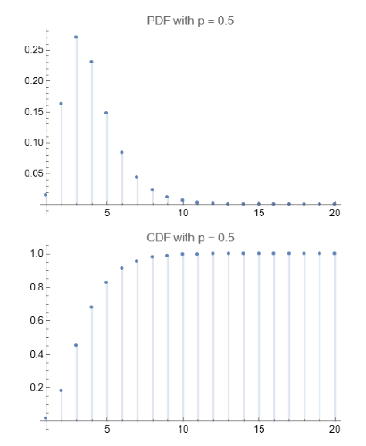
Visualize the mass and density function for the discrete distribution:
In[]:=
GraphicsColumn@{DiscretePlot[PDF[,t],{t,1,20},PlotLabel->"PDF with p = 0.5"],DiscretePlot[CDF[,t],{t,1,20},PlotLabel->"CDF with p = 0.5"]}
Out[]=
I can also generate the distribution function given known CDF function of the underlying model:
In[]:=
Clear[n,p]
In[]:=
p=ProbabilityDistribution[{"CDF",(1-(1-p)^n)^6},{n,1,Infinity,1},Assumptions->0<p<1]//FullSimplify;
In[]:=
m2=Mean[]//FullSimplify
Out[]=
1
60
685
-2+p
147
p
390(-3+p)
3+(-3+p)p
450
2+(-2+p)p
10(1+p)
1+(-1+p)p
720-72p(10+(-5+p)p)
5+p(-10+p(10+(-5+p)p))
Verify the expression for or 50%:
p=1/2
In[]:=
{#,N[#]}&[m2/.p->1/2]
Out[]=
,4.03482
7880
1953
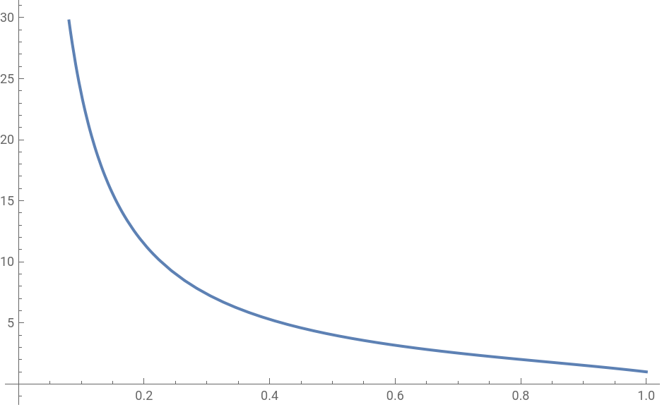
The mean value changes with
In[]:=
Plot[m2,{p,0,1}]
Out[]=
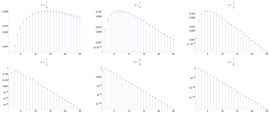
PDF with different value of :
p
In[]:=
pList={1/8,1/4,1/3,1/2,3/4,7/8};pdfs=PDF[p/.p->#,t]&/@pList;
In[]:=
GraphicsGrid[Partition[MapThread[DiscretePlot[#1,{t,1,25},ScalingFunctions->"Log",PlotLabel->Row[{"p = ",#2}],ImageSize->400]&,{pdfs,pList}],3],ImageSize->1200]//Rasterize[#,ImageResolution->800]&
Asymptotic behavior
Asymptotic behavior
◼
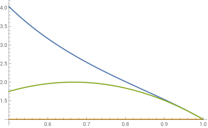
p approaches 1 to first and second order. The asymptotics are flat line and a parabola:
In[]:=
Asymptotic[m2,{p,1,#}]&/@{1,2}
Out[]=
{1,-2+12p-9}
2
p
Visualize the behavior across predefined domain:
In[]:=
Plot{m2,1,-2+12p-9},{p,0.5,1},PlotLegends->{"Mean","1st order asymp.","2nd order asymp."}
2
p
Out[]=


◼
p approaches 0 to first and second order. The asymptotic line is hyperbola:
In[]:=
Asymptotic[m2,{p,0,#}]&/@{1,2}
Out[]=
,-+--
49
20p
29
40
49
20p
49p
240
49
2
p
480
Plot the second order approximation over the mean value:
Exam the function of mean of D on the complex plane:
Discrete Markov process
Discrete Markov process
Markov process might be overkill for this problem. But this tool is extremely powerful if the probability of seed growth is not constant in some case. The transition matrix is powerhouse to store the parameters of any kind. Lets first show how to create the transition matrix for our particular case:
Assume we have 6 seeds again. If we encode
◼
seed not yet grow into flower as 0
◼
seed grows to flower: 1
Generate Markov transition matrix and path graph by binarizing the states we have sofar:
Create the transition matrix with SparseArray
The above graph is likely a familiar object to most Mathematica users:
In[]:=
Sierpiński triangle
Sierpiński’s triangle (Pascal’s triangle mod 2) converted to decimal.
In[]:=
oeis A001317
Find the Markov process with initial state and transition matrix:
Compute the process given the transition matrix:
Create a random function based on the process:
Find the characteristic function for this distribution:
In[]:=
Characteristic Function
The stationary is clearly when all seeds grow into flower {0,0,0,0,0,0} -> {1,1,1,1,1,1} = 64:
The process can also be visualize with the connection graph between the states:
Or setting GraphLayout to none to eliminate the output graph plot:
I can probe into the graph to see if some states can be reached from a given one. For instance node with 6th state = 5 with DFS scan
A quick remark is that the complexity of the DFS tree depends on the number of 0 in the binary form of the number. More zeros = more reachable states and longer chain:
Compare to:
Summary
Summary
This demo shows the tight integration of the different branches of knowledge and technology to help understanding the classic problem. I use many built-in functions to explore the details of the process with pure symbolic computation, Markov process, graph and finally relate to the famous Sierpinski triangle. The journey filled with experiments and simulation is much more pleasant than just dry mathematical derivation. Hopefully the reader enjoys the article and find their wolfram way to learn probability and statistics.
CITE THIS NOTEBOOK
CITE THIS NOTEBOOK
Six seeds problem, Markov and Sierpiński
by Shenghui Yang
Wolfram Community, STAFF PICKS, November 1, 2023
https://community.wolfram.com/groups/-/m/t/3059225
by Shenghui Yang
Wolfram Community, STAFF PICKS, November 1, 2023
https://community.wolfram.com/groups/-/m/t/3059225