ABSTRACT (original article): We present a method for constructing global analytical expressions that approximate a function over its entire range. These approximations not only mirror the original function as accurately as desired, but are purposefully created to possess features that the original function lacks. This is particularly useful for functions that lack closed form and are defined by integrals or infinite series. Replacing these definitions with simple analytical expressions enables in-depth qualitative analysis and replaces the current methods of evaluation. We demonstrate this procedure by providing replacements for a variety of pivotal functions in physics and cosmology including the pressure and density of quantum gas, the one-loop correction in thermal field theory, common polylog functions, and the error function. CITATION (original article): Aviv Orly (2024), Analytical approximations as close as desired to special functions, arXiv:2406.11947. https://doi.org/10.48550/arXiv.2406.11947
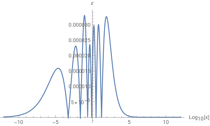
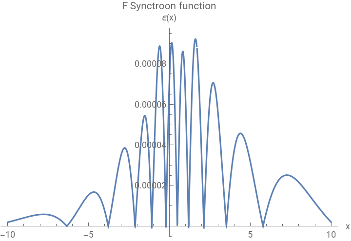
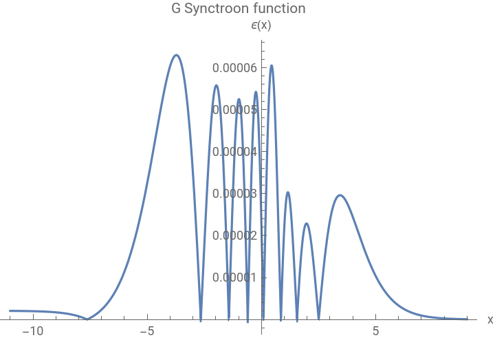
This notebook analyzes analytical approximations for various important special functions that lack an analytical form. We plot the relative residuals for each function between its given approximation and its full numerical calculation.For each function, we plot its relative error, ϵ, which is defined by:The idea is that whenever ϵ is an order of magnitude smaller than the required precision or error, the analytical approximation can safely replace the usage of the original function from the point of view of any practical consideration. Thus, using the approximation can replace numerical calculations and substantially accelerate computations. Moreover, these analytical expressions can be used to expand full analytical capabilities by replacing numerical methods or long, limited range expansions.
ϵ≡-
f
approximation
f
numerical
f
numerical
TheModifiedBesselFunctionoftheSecondKindK2
TheModifiedBesselFunctionoftheSecondKind
K
2
We define the analytical approximation of the Bessel Function of the Second Kind , valid for 0≤x≤∞, then plot its relative error.
K
2
In[]:=
k2App[x_,c0_]:=Exp[-x]*SetPrecision(1+2.627/x+2/x^2),100ϵ[x_]:=Abs1-PlotϵSetPrecision,100,{logx,-12,12},PlotRangeAll,AxesLabel{"[x]","ϵ"}
1
2c0
(0.033*x^(c0/5)-0.102*x^(c0/4)+0.113*x^(c0/3)+1.162*x^(c0/2)+(2*x/π)^c0+1)
k2App[x,1.984]
BesselK[2,x]
logx
10
Log
10
Out[]=
Synchrotron function
Synchrotron function
The two Synchrotron functions F,G are defined by:We plot their relative error, ϵ, in the approximated range of 0≤x≤∞:
F(x)≡x(t)t
∞
∫
x
K
5
3
G(x)≡x(x)
K
2
3
δ=30;Fapp[x_]:=SetPrecision(230/107*x^(1/3)+x-0.7078*x^0.701)2.835*x^0.61264-0.967*x^0.3792-0.701*x^0.8239-0.61264*x^0.89696+^1.1843+1^0.42219,100smallF[x_]:=xNIntegrateBesselK,t,{t,x,∞},AccuracyGoal15,WorkingPrecision15,MinRecursion5,MaxRecursion20expansion=SimplifyyNormalSeriesBesselK,t,{t,∞,10}t,Assumptionsy>0;largeF[x_]:=expansion/.yx;(*AsthecomplexityofthenumericalintegrationthatevaluetesthefunctionFgreatlyincreasesthelargerxis,abovex~50wemustembracedifferentstrategies.Forthat,weseriesexpandFtogetitsfirst10termsaroundx=∞.Thenweswitchbetweennumericalintegrationtoseriesexpansionatx=50*)F[x_]:=If[x<50,smallF[x],largeF[x]]Fapp[x_]:=SetPrecision[,δ]SetPrecision(230/107*x^(1/3)+x-0.7078*x^0.701)2.835*x^0.61264-0.967*x^0.3792-0.701*x^0.8239-0.61264*x^0.89696+^1.1843+1^0.42219,δϵ[x_]:=Abs1-Plot[ϵ[SetPrecision[10^logx,δ]],{logx,-10,10},PlotRangeAll,PlotLabel"F Synchrotron function",AxesLabel{"(x)","ϵ"}]
-x
2x
π
5
3
∞
∫
y
5
3
-x
2x
π
Fapp[x]
F[x]
Log
10
Out[]=
G[x_]:=xBesselK,xGapp[x_]:=SetPrecision+x,δϵ[x_]:=Abs1-PlotAbsϵSetPrecision,δ,{logx,-11,9},PlotRangeAll,PlotLabel"G Synchrotron function",AxesLabel{"x","ϵ(x)"}
2
3
-x
115
107
1
3
x
19
108
3.96+4.815+1.74++1
0.6366
x
1.425
x
2.1711
x
54
19
2x
π
Gapp[x]
G[x]
logx
10
Out[]=
Polylog
Polylog
We want to approximate to Polylogarithm function, (x), for varies important rational s values.For that we define the analytical approximation model f[x, s, cRow], which gets a specific s value and its corresponding model coefficients from the table constantsMatrix. With that we create a table that represents the maximal relative error , for each of the s values: ,,,,,,2,,3,,4,,5,,6,.
LI
s
,
ϵ
max
1
3
1
2
2
3
4
3
3
2
5
3
5
2
7
2
9
2
11
2
13
2
constantsMatrix=
;
5 | -1.2 | 0.49 | 663 | -227 | 3.371 | 139 | -10.5 | 46 | 236 | 9.7 | 286 | -10 | -1.66 |
7.7 | -0.67 | 0.057 | 473 | -23 | 3.376 | 58 | -7.4 | -212 | 241 | 9 | 312 | -11 | -1.24 |
11.8 | -1.1 | 0.09 | 519 | 28 | 3.58 | 57 | -5.2 | -547 | 255 | 7.9 | 346 | -12.7 | -1.13 |
1.4732 | 0.125 | 0.00198 | 5.4 | 12.1 | 1.02 | 10.84 | 4.37 | 13 | 135.1 | 11.79 | 404 | -10.8 | -1.885 |
1.52 | 0.0964 | 0.0011 | 15.35 | 28.15 | 1.1931 | 20 | 6.596 | -94.5 | 131.8 | 11.86 | 443.67 | -11.46 | -2.152 |
3.02 | 0.196 | 0.0093 | 37.8 | 57.3 | 0.9295 | 33.17 | 8.74 | 50.6 | 116 | 12 | 476 | -11.8 | -1.283 |
24 | -0.17 | 0.128 | 100.8 | 132 | 0.5685 | 63.5 | 13.14 | 300 | 88.6 | 11.6 | 541 | -13 | -0.775 |
32.2 | 38.7 | 38.8 | 9.75 | 22.3 | 1.206 | 13 | 6.82 | 103.6 | 71.7 | 10 | 651 | -15.3 | 0.12638 |
26.569 | 26.69 | 15.88 | 34.7 | 62.38 | 0.253 | 27.33 | 10.18 | 633.79 | 30.8 | 7.64 | 681.3 | -17.2 | 0.25076 |
42.95 | 36.9 | 12.34 | 85.5 | 122.17 | 1.197 | 49.79 | 12.114 | 516.26 | 19.4 | 5.8 | 768.2 | -20.8 | 0.3759 |
103.84 | 92.24 | 19.97 | 26.76 | 17.39 | 7.02 | 13.8 | 3.58 | -164 | 33 | 5.4 | 1050 | -27 | 0.50028 |
9.774 | 2.909 | 0 | 235 | 326 | 0.091 | 126.2 | 15.65 | 715.8 | -16.4 | 2.6 | 711.8 | -28 | 1.25 |
70.4 | 60.6 | 8.25 | 1855 | 836 | 3 | 179 | 14.3 | 202 | -19 | 1 | 229 | -24.6 | 0.7488 |
149 | 76.3 | 4.63 | 1012 | 887 | -34.2 | 284 | 28.3 | 342 | -29.9 | 1.36 | 206 | -18.8 | 0.8758 |
233.98 | 112.86 | 7.98 | 10.3 | 11 | -1 | 7 | 1.81 | 2004 | -24 | 2.8 | 1981 | -30 | 1.00017 |
280.6 | 122.3 | 5.132 | 22 | 20 | -82 | 9 | 22.7 | 809 | -48 | 1.3 | 629 | -39 | 1.124 |
Error function
Error function
Fermi&Bose gas number density
Fermi&Bose gas number density
Fermi&Bose gas number density
Fermi&Bose gas number density
Fermi gas pressure
Fermi gas pressure
Fermi&Bose gas pressure
Fermi&Bose gas pressure
Fermi gas pressure with chemical potential
Fermi gas pressure with chemical potential
CITE THIS NOTEBOOK
CITE THIS NOTEBOOK
Analytical approximations as close as desired to special functions
by Aviv Orly
Wolfram Community, STAFF PICKS, July 9, 2024
https://community.wolfram.com/groups/-/m/t/3208909
by Aviv Orly
Wolfram Community, STAFF PICKS, July 9, 2024
https://community.wolfram.com/groups/-/m/t/3208909