Saint Francois Mountains of Southeast Missouri
Saint Francois Mountains of Southeast Missouri
A few days ago, some friends of mine visited an area of southeast Missouri and posted some pictures of the surrounding rocks that looked odd to me for something found in the mid-west United States. Normally, any exposed rocks in the mid-west United States are sedimentary rocks like limestone or maybe sandstone, but the rocks in their pictures were obviously igneous, having formed from magma that cooled deep underground. These rocks are part of the Saint Francois Mountains which are shown as isolated red points in the southeast corner of the following map.
In[]:=
GeoGraphicsEdgeForm[Directive[Black,Thickness[.005]]],FaceForm[],Polygon,Red,Point/@EntityList,GeoRange->,GeoBackground->"ReliefMap"

Out[]=
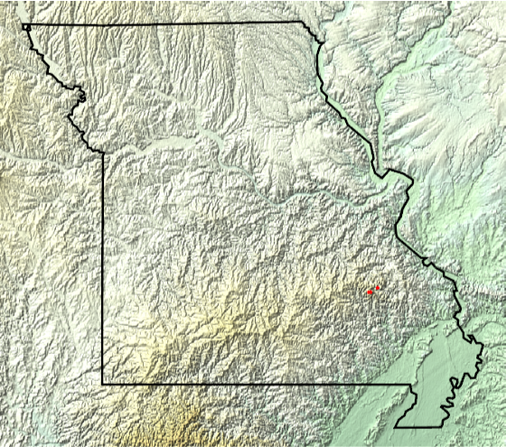
The above map shows the location, but the area can be explored further from a more geological point of view. Let’s strip away all of the soil and plot the bedrock in the area of these mountains. The rocks in this area can be dated to the Mesoproterozoic Era.
In[]:=
GeoGraphicsEdgeForm[Directive[Black,Thickness[.005]]],FaceForm[],Polygon,GeoStyling[Red],,GeoRange->,GeoBackground->"ReliefMap"
Out[]=
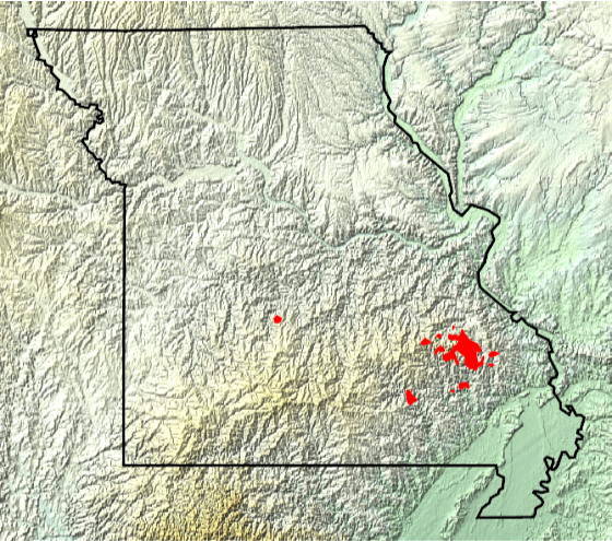
For additional context, we can plot the bedrock in the surrounding area. A Wolfram Function Repository (WFR) item can make this a bit easier. The Mesoproterozoic area from above can be seen as tan color and is surrounded immediately by rocks that are Cambrian in age and the rocks get younger as we move away from the mountains.
In[]:=
Out[]=
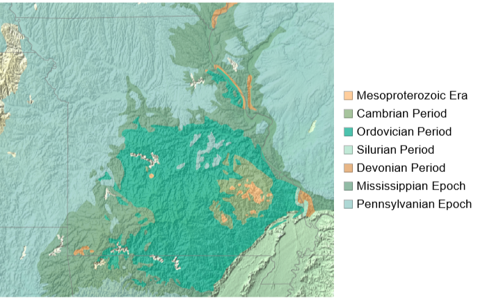
Perhaps not obvious to the geologically uninitiated, but there is a big time gap between the Mesoproterozoic Era and the Cambrian Period.
In[]:=
EntityValue,,"TimeRange"
Out[]=
,
Using another WFR item we can visualize the time periods involved. In the following chart, the Cambrian Period would be at the very top edge. The Mesoproterozoic Era is part of the Precambrian. There is nearly 1 billion years of age difference between the rocks of the Saint Francois Mountains and the surrounding Cambrian rocks.
Out[]=
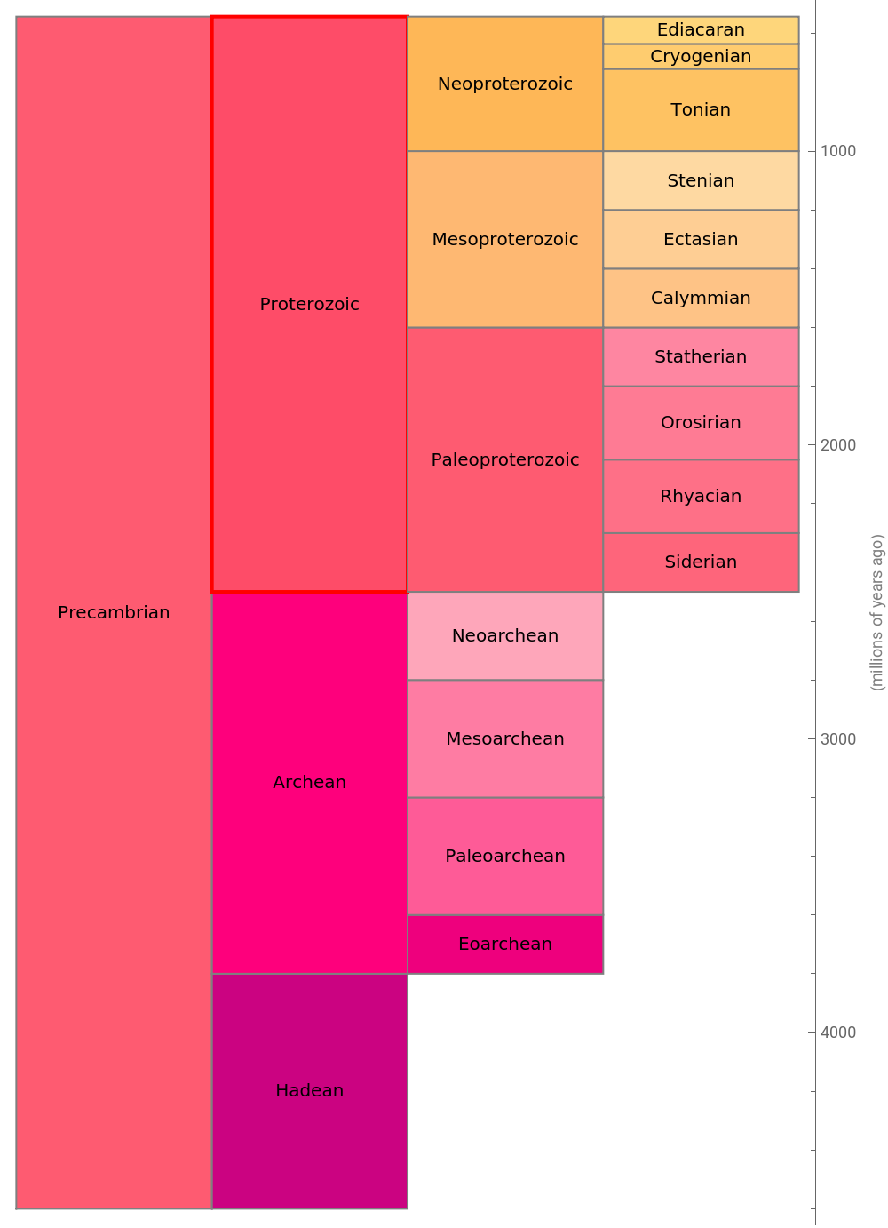
Typically when looking at rock layers, there is a consistent difference in age as you move up or down in the rock layers. Older rocks are lower and younger rocks are above them with a slow gradual transition from older to younger as you go up. In geology, when you have rocks that are overlain or that are in contact with other rocks of a radically different age, this is known as an unconformity. This particular large gap is known as the Great Unconformity and can be found in rocks all around the world where rocks of these ages are exposed. The Grand Canyon in the southwestern United States is famous for its exposure of the Great Unconformity.
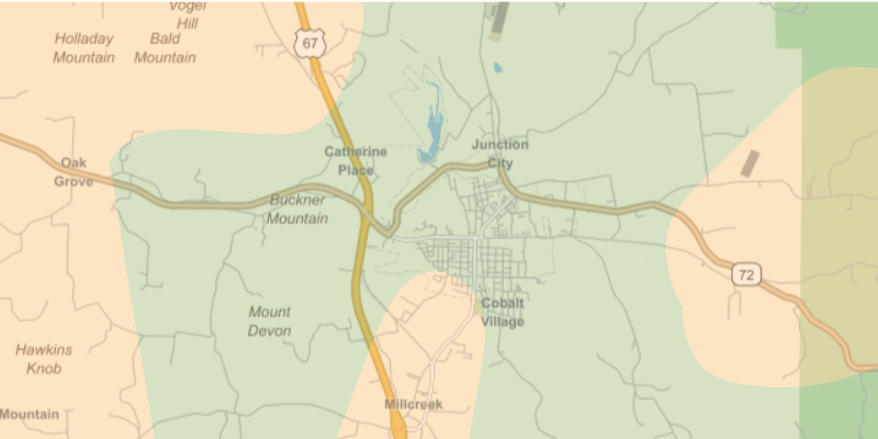
Some good places to observe the Great Unconformity in Missouri are along road cuts in the Fredericktown area. Overlaying the bedrock colors on top of a street map, we can see places where the older Mesoproterozoic rock (shown in tan) butts up against the younger Cambrian rock (shown in green). West of Frederickstown along highway 72 and also south of town along highway 67 are reportedly good places to observe the Great Unconformity which seems to agree with the geologic map shown below.
In[]:=
Out[]=
Exploring the Basement Rocks
Exploring the Basement Rocks
Up until now, the bedrock that lies just under the soil across Missouri has been explored. But what if we go deeper and strip away all of the overlying sedimentary rocks that were created by erosion of older rock and deposition of sandstone and shale and deposition by living creatures such as limestone? The Saint Francois Mountains in Missouri exposes a small portion of this crystalline basement rock, but what about across the rest of the United States? We want to explore the core of the continent and its various ages and domains.
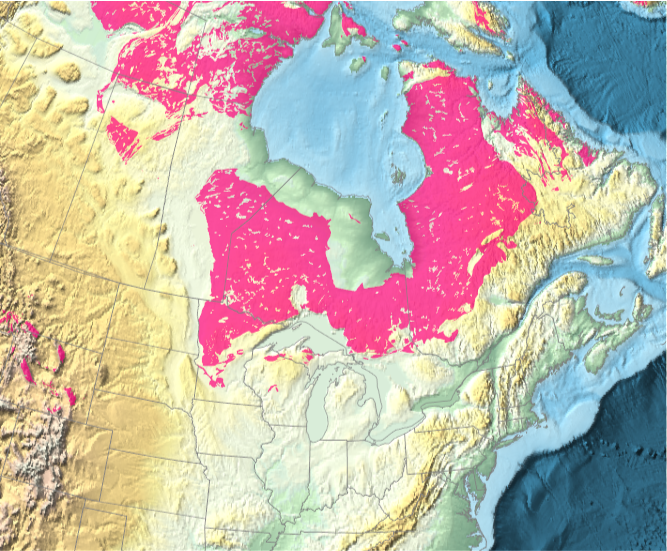
A portion of this ancient basement rock represents the bedrock in the Canadian Shield and is even exposed at the surface in some of those areas. Only a portion of this extends into the United States in parts of Minnesota and a few places in Wisconsin and localized outcrops in the Rocky Mountains in Wyoming.
In[]:=
Out[]=
To explore this basement rock in the rest of the United States, we need new data since it underlies the younger bedrock.
Data Processing
Data Processing
I found some relevant data in “Basement Domain Map of the Conterminous United States and Alaska” by Karen Lund, S.E. Box, C.S. Holm-Denoma, C.A. San Juan, R.J. Blakely, R.W. Saltus, E.D. Anderson, and E.H. DeWitt. The publication included online data in the form of Shape files.
As is the case with most real-world data, it requires a bit of work to make the data computable. Some of the data contains <Null> and contains values without units explicitly specified. The following takes care of these issues and converts the data into rules.
With the data extracted, we want to align it to specific geological periods so we can associate the data with standardized colors. First we need to setup a set of rules to associate geological periods with their time ranges.
Now, we can associate the formation age (which is a mix of explicit date ranges as strings as well as named geological periods as strings) from the new data with the GeologicalPeriod entity type so we can obtain the standard color for that period and create a new list of rules associating the “fuzzy” formation age strings from the new data with a best attempt at standardized color.
Its also useful to generate some political boundaries of the United States for reference.
We also need to generate the geo primitives and give them distinct colors and tooltips as useful annotations.
How the domains will be colored depends on preference. The following generates the necessary primitives, but is dependent on the color rules requested.
Now I assemble the map of the lower 48 U.S. states.
From the assembled map, its useful to try ways of annotating the results. I start by extracting the annotations that were added to the primitives.
From these annotations, I can construct centroids for each polygon.
Here, I do a similar set of operations for Alaska.
Create Map
Create Map
With all of the elements assembled, now we can create various map variants that cover the United States, including Alaska. To provide as much detail as possible, I’ve actually divided the result into two different map types, ones for the contiguous United States and separate ones for Alaska. The maps showing the contiguous United States are more relevant as an extension of the previous discussion.
The first map variant relies on tooltips for each region so that you can see a variety of data for each domain without worrying about collisions between all the data being shown at the same time. One downside to this approach is that if you rasterize the results (like what happens automatically for GeoGraphics in cloud environments), then you don’t get access to the non-geometric data. But for desktop users, this presents the optimal form.
Color the map according to standardized age of the corresponding geological period:
Color the map according to an arbitrary ColorData indexed color scheme (this scheme will be used for the rest of the examples). There are only 15 unique colors in this scheme so colors will repeat using this approach:
The second variant relies on callouts to label each domain. Even when the name of the domain is the only data being shown, its not easy to avoid collisions. Only some of the domains have explicit callouts, the others fall back to tooltips since they are too crowded.
Trying to present all of the data per domain as part of the callout makes the problem worse. Even fewer domains have an explicit callout because collisions are even harder to avoid.
Similarly, I have explored Alaska along the same lines as above.
Of course if you really want to see all the non-geometric data, it can be extracted and presented as a dataset.
The static maps are nice to look at and do have tooltips describing the formation dates of the various geological domains, but for more clarity, we can interactively animate the various domains in time and show how the Unites States was assembled.
It would be even more useful if the data had more complete coverage of the accretion time in addition to the formation time. The accretion time would better represent when the various domains were sutured to the growing core of the North American continent. The formation dates do a decent job, but keep in mind that a given domain may form elsewhere, long before it ever gets sutured to North America. For example, a domain may form long ago on a distant ancient continent, later it rifts apart and drifts across the ocean and then, much later, sutures itself onto North America. For example, the Carolinas formed 670 million years ago (somewhere else), but didn’t get accreted onto North America until the Devonian Period about 400 million years ago. So, it spent over 200 million years elsewhere before being accreted and sutured to North America.
CITE THIS NOTEBOOK
CITE THIS NOTEBOOK
The Geologic Assembly of the United States
by Jeff Bryant
Wolfram Community, STAFF PICKS, July 6, 2023
https://community.wolfram.com/groups/-/m/t/2952971
by Jeff Bryant
Wolfram Community, STAFF PICKS, July 6, 2023
https://community.wolfram.com/groups/-/m/t/2952971