The study of the dynamics of the discrete Klein - Gordon equation (DKG) with friction is given by the equation :
̈
U
n
U
n+1
U
n
U
n-1
U
n
′
W
U
n
In the above equation, describes the potential function:
W
W()-+
U
n
2
w
d
2
2
U
n
β
2
w
d
4
4
U
n
to which every coupled unit adheres. In Eq. (1), the variable (t) is the unknown displacement of the oscillator occupying the -th position of the lattice, and is the discretization parameter. We denote by the distance between the oscillators of the lattice. The chain (DKG) contains linear damping with a damping coefficient , while is the coefficient of the nonlinear cubic term.
U
n
U
n
n
k
-2
h
h
δ>0
β
For the DKG chain (1), we will consider the problem of initial-boundary values, with initial conditions
U
n
U
n,0
U
n
U
n,1
K+2
R
and Dirichlet boundary conditions at the boundary points -L/2 and L/2, that is,
x
0
x
K+1
U
0
U
K+1
Therefore, when necessary, we will use the short notation for the one-dimensional discrete Laplacian
Δ
d
{U}
Δ
d
n∈Z
U
n+1
U
n
U
n-1
In this note book, we investigate numerically the dynamics of the system (1)-(2)-(3). Our first aim is to conduct a numerical study of the property of Dynamic Stability of the system, which directly depends on the existence and linear stability of the branches of equilibrium points.For the discussion of numerical results, it is also important to emphasize the role of the parameter . By changing the time variable , we rewrite Eq. (1) in the form-U+-β, t>0, , hδThe change in the scaling of the lattice parameter of the problem makes it important to comment here on the nature of the continuous and anti-continuous limit. For the anti-continuous limit, we need to consider the case in Eq. (1) where ∞. In the case of nonlinearity present in the governing equations, the continuous limit needs to be taken as well. On the other hand, for small values of the parameter, the system becomes significant. However, because of the model we consider, we take the asymptotic linear limit as 0.
2
ω
d
t
t
h
̈
U
n
Δ
d
δ
U
n
2
Ω
d
U
n
3
U
n
2
Ω
d
2
h
2
ω
d
δ
2
ω
d
2
ω
d
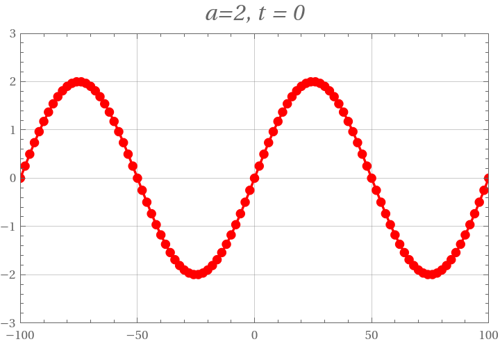
We consider spatially extended initial conditions of the form :
U
n
U
n,0
jπhn
L
where is the distance of the grid and is the amplitude of the initial condition .We also assume zero initial velocity:
h
L
K+1
a>0
U
n
U
n,1
In[]:=
ClearAll["Global`*"]
L=200;(*Lengthofthesystem*)k=99;(*Numberofspatialpoints*)j=2;(*Modenumber*)aInit=2;(*Exampleinitialamplitudefortheinitialconditionplot*)(*spatialgrid*)h=L/(k+1);n=Subdivide[-L/2,L/2,k+1];(*Spatialpoints*)
In[]:=
(*Initialpositions*)u0Init=aInit*Sin[(j*Pi*h*n)/L];
In[]:=
(*Createtheplot*)initialConditionPlot=ListLinePlotTranspose[{n,u0Init}],PlotStyle->{Red,PointSize[Medium],Thickness[0.005]},Mesh->All,MeshStyle->PointSize[0.02],AxesLabel->Style"x._n",Italic,16,Style"u._n",Italic,16,PlotLabel->Style["a=2, t = 0",Italic,16],BaseStyle->{FontSize->12,FontFamily->"Times"},PlotRange->{{-L/2,L/2},{-3,3}},GridLines->Automatic,PlotTheme->"Scientific";(*Displaytheplot*)initialConditionPlot
Out[]=
In[]:=
ClearAll["Global`*"]
(*parameters*)a=2;(*Amplitudeoftheinitialcondition*)j=2;(*Modenumber*)L=200;(*Lengthofthesystem*)k=99;(*numberofspatialpoints*)omegad=1;(*characteristicfrequency*)beta=1;(*Nonlinearityparameter*)
(*dampingcoefficient*)delta=0.05;
(*spatialgrid*)h=L/(k+1);n=Subdivide[-L/2,L/2,k+1];(*Spatialpoints*)
(*discretizationparameter*)kappa=h^-2;
(*Scaledparameters*)omegad2=(h^2)*omegad^2;deltaHat=h*delta;
tmax=3000;(*Maximumtime*)dt=0.05;(*Timestep*)tspan=Range[0,tmax,dt];(*Timevector*)
(*Initialpositions*)initialPositions=a*Sin[Pi*j*n*h/L];