Lecture Notebooks for Vector Calculus
Lagrange multipliers
By Passant Abbassi
Wolfram Summer School 2022
passant.abbassy@guc.edu.eg
Project Mentors: Paul Abbott and Daniel Robinson, Wolfram Research
Lagrange multipliers
By Passant Abbassi
Wolfram Summer School 2022
passant.abbassy@guc.edu.eg
Project Mentors: Paul Abbott and Daniel Robinson, Wolfram Research
Motivation
Motivation
Many problems in Engineering and science require us to find the maximum or minimum of a differentiable function f. The scope of the project is to create a lecture notebook on Lagrange multipliers. The main aim is to make good use of lecture notebooks in the classroom by including live interactive content that can be altered—and even extended, while presenting. This lets classes be truly dynamic and provides an unparalleled opportunity to involve students in the content creation.
Method of Lagrange Multipliers
Method of Lagrange Multipliers
Optimization with a constraint for functions of two or three variables
Optimization with a constraint for functions of two or three variables
How do you implement Lagrange multipliers?
1
.Compute gradient: f(x,y),g(x,y),,,
∇
{x,y}
∇
{x,y}
f
x
f
y
g
x
g
y
2
.Apply lagrange multipliers: f(x,y)=λg(x,y)⟹=λ,=λ
∇
{x,y}
∇
{x,y}
f
x
g
x
f
y
g
y
3
.Solve the 3 equations =λ,=λ,g(x,y)=k and 3 unknowns to get the critical points
f
x
g
x
f
y
g
y
(x,y,λ)
4
.Plug the critical points in the function to identify max and min values: The point that gives largest value of function is Absolute maximum while the point that gives smallest value of function is Absolute minimum.
f(x,y)
f(x,y)
f(x,y)
As an example, let’s find the extreme values of subject to the constraint .
f(x,y)
g(x,y)=k
Example 1: Find extreme values of f(x,y)=2x+22y subject to the constraint g(x,y)=2x+2y
Example 1: Find extreme values of subject to the constraint
f(x,y)=+2
2
x
2
y
g(x,y)=+
2
x
2
y
In this example, subject to the constraint .
f(x,y)=+2
2
x
2
y
g(x,y)=+
2
x
2
y
In[]:=
f[x_,y_]:=+2
2
x
2
y
In[]:=
g[x_,y_]:=+
2
x
2
y
To find the maximum and minimum values of subject to the constraint , apply Lagrange multipliers.
f(x,y)
g(x,y)=k
Find all values of and such that:
x,y
λ
∇
{x,y}
∇
{x,y}
f
x
g
x
f
y
g
y
1
.Compute gradient:
In[]:=
gradf=f[x,y]
∇
{x,y}
Out[]=
{2x,4y}
In[]:=
gradg=g[x,y]
∇
{x,y}
Out[]=
{2x,2y}
2
.Apply Lagrange multipliers:
In[]:=
∇
{x,y}
∇
{x,y}
Out[]=
{2x,4y}{2xλ,2yλ}
In[]:=
lagrange=Thread[Equal[{2x,4y},{2xλ,2yλ}]]//Column
Out[]=
2x2xλ |
4y2yλ |
In[]:=
(system=Flatten[{lagrange,g[x,y]1}])//Column
Out[]=
16x8xλ |
4z2yλ |
-16+4y8zλ |
2 x 2 y |
3
.Solve the 3 equations and 3 unknowns to get the critical points:
In[]:=
Solve[system,{x,y,λ}]
Out[]=
{{x0,y-1,λ-1},{x0,y1,λ-1}}
Equation (1) implies that or .
x=0
λ=1
◼
If , then equation (3) implies that . This yields 2 points
x=0
y=±1
(0,±1)
◼
If , then equation (2) implies that and by equation (3), . This yields 2 points
λ=1
y=0
x=±1
(±1,0)
4
.Plug the critical points in the function to identify max and min values:
f(x,y)
Now evaluating at the 4 points and
f(x,y)
(±1,0)
(0,±1)
◼
f(±1,0)=1
f(0,±1)=2
5
.Conclusion:
◼
f(x,y)
(0,±1)
◼
f(x,y)
(±1,0)
Visualize the functions and their contour plots
Visualize the functions and their contour plots
Plot of function :
f(x,y)
In[]:=
plot3D=Plot3D[f[x,y],{x,-1.5,1.5},{y,-1.5,1.5},PlotLabelStyle["f(x,y)=+2",18,Bold,Red]]
2
x
2
y
Out[]=

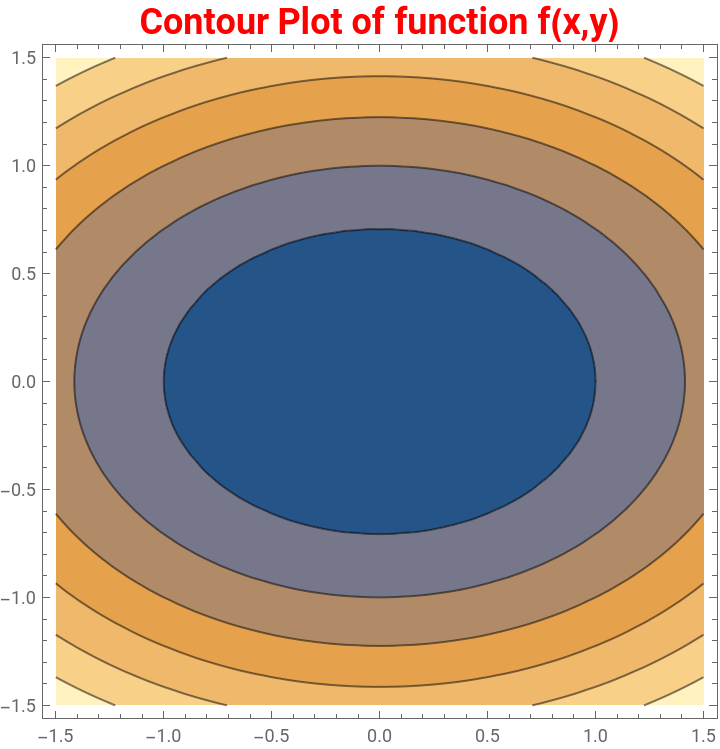
Contour Plot of function :
f(x,y)
In[]:=
fplot=ContourPlot[f[x,y],{x,-1.5,1.5},{y,-1.5,1.5},PlotLabelStyle["Contour Plot of function f(x,y)",18,Bold,Red]]
Out[]=
Example 2: Find the minimum distance from the surface 2x-2y-2z=1 to the origin
Example 2: Find the minimum distance from the surface --=1 to the origin
2
x
2
y
2
z
We wish to minimize the value of function for points on the surface --=1. Equivalently, the problem may be formulated as finding the minimum of squared distance from the origin subject to the constraint .
d(x,y)=++=++
2
(x-0)
2
(y-0)
2
(z-0)
2
x
2
y
2
z
(x,y,z)
2
x
2
y
2
z
d(x,y)=++
2
x
2
y
2
z
g(x,y,z)=--=1
2
x
2
y
2
z
In[]:=
d[x_,y_,z_]:=++
2
x
2
y
2
z
In[]:=
g[x_,y_,z_]:=--
2
x
2
y
2
z
To find the minimum values of subject to the constraint , apply the Lagrange multipliers.
d(x,y,z)
g(x,y,z)=k
In other words, find all values of and such that:
x,y,z
λ
∇
{x,y}
∇
{x,y}
f
x
g
x
f
y
g
y
f
z
g
z
1
.Compute gradient:
In[]:=
gradd=Grad[d[x,y,z],{x,y,z}]
Out[]=
{2x,2y,2z}
In[]:=
gradd=Grad[g[x,y,z],{x,y,z}]
Out[]=
{2x,-2y,-2z}
2
.Apply Lagrange multipliers:
In[]:=
∇
{x,y,z}
∇
{x,y,z}
Out[]=
{2x,2y,2z}{2xλ,-2yλ,-2zλ}
In[]:=
lagrange=Thread[Equal[{2x,2y,2z},{2xλ,-2yλ,-2zλ}]];lagrange//Column
Out[]=
2x2xλ |
2y-2yλ |
2z-2zλ |
3
.Solve the 4 equations and 4 unknowns to get the critical points:
In[]:=
system=Join[lagrange,{g[x,y,z]1}];system//Column
Out[]=
2x2xλ |
2y-2yλ |
2z-2zλ |
2 x 2 y 2 z |
Reduce will return a set of equations equivalent to the input. Solve will try to find a solution (it makes more assumptions).
Example 3: Hottest point on space probe’s surface
Example 3: Hottest point on space probe’s surface
Find the hottest point on the probe's surface.
1
.Compute gradient:
2
.Apply Lagrange multipliers:
3
.Solve the 4 equations and 4 unknowns to get the critical points: