Study a 1-dimensional quantum system confined in the potential if and otherwise:
V(x)=mgx
x>=0
V(x)=∞
-ψ+mgxψ=ℏwithψ(0,t)=0
2
ℏ
2m
2
∂
∂
2
x
∂ψ
∂t
(
1
)◼
Find eigenstates and eigenvalues
◼
Simulate the time evolution
Find Eigenstates
Find Eigenstates
Perform a variable substitution using the transformation , applicable to the context of a quantum particle within a gravitational potential field:
x->z
1/3
2
ℏ
2g
2
m
In[]:=
DSolveChangeVariablesInactive[DSolve]-u''[x]+mgxu[x]==Εu[x],u[x],x,ψ,z,x==z//Simplify
2
ℏ
2m
1/3
2
ℏ
2g
2
m
Out[]=
DSolveΕψ[z],ψ[z],z
gm(zψ[z]-[z])
1/3
2
ℏ
g
2
m
′′
ψ
1/3
2
Transform the equation into a dimensionless form by substituting variables and redefining energy as with =:
ε=
Ε
mg
x
0
x
0
1/3
2
ℏ
2g
2
m
In[]:=
DSolve[-[z]+zψ[z]εψ[z],ψ[z],z]
′′
ψ
Out[]=
{{ψ[z]AiryAi[z-ε]+AiryBi[z-ε]}}
1
2
Identify the appropriate limits to ensure the wavefunction remains well behaved and eliminates divergent terms by imposing physical boundary conditions and constraints:
In[]:=
Limit[AiryAi[z],z->∞]Limit[AiryBi[z],z->∞]
Out[]=
0
Out[]=
∞
Impose the limits to ensure the wavefunction adheres to physical constraints and apply energy quantization conditions to determine the discrete allowed energy levels:
In[]:=
Reduce[AiryAi[-ε]==0,ε,Reals]
Out[]=
1
1
1
Find the leading asymptotic approximation of higher energies:
In[]:=
Asymptotic[AiryAiZero[n],{n,∞,1}]
Out[]=
-
1
4
2/3
(-1+4n)
2/3
(3π)
Find the normalization constant:
In[]:=
f=Integrate[,z]//FullSimplify
2
AiryAi[z+AiryAiZero[n]]
Out[]=
-+(z+AiryAiZero[n])
2
AiryAiPrime[z+AiryAiZero[n]]
2
AiryAi[z+AiryAiZero[n]]
In[]:=
FullSimplify[Limit[f,z->0],Assumptions->n∈PositiveIntegers]
Out[]=
-
2
AiryAiPrime[AiryAiZero[n]]
In[]:=
Limit[f,z->∞]
Out[]=
0
Define the normalized eigenstates:
In[]:=
ps[n_]:=
AiryAi[z+AiryAiZero[n]]
Abs[AiryAiPrime[AiryAiZero[n]]]
Check orthonormality of some eigenstates:
In[]:=
Withlist=Table,{n,10},Outer[Quiet@NIntegrate[#1#2,{x,0,∞}]&,list,list]//Chop//MatrixForm
AiryAi[x+AiryAiZero[n]]
Abs[AiryAiPrime[AiryAiZero[n]]]
Out[]//MatrixForm=
1. | 0 | 0 | 0 | 0 | 0 | 0 | 0 | 0 | 0 |
0 | 1. | 0 | 0 | 0 | 0 | 0 | 0 | 0 | 0 |
0 | 0 | 1. | 0 | 0 | 0 | 0 | 0 | 0 | 0 |
0 | 0 | 0 | 1. | 0 | 0 | 0 | 0 | 0 | 0 |
0 | 0 | 0 | 0 | 1. | 0 | 0 | 0 | 0 | 0 |
0 | 0 | 0 | 0 | 0 | 1. | 0 | 0 | 0 | 0 |
0 | 0 | 0 | 0 | 0 | 0 | 1. | 0 | 0 | 0 |
0 | 0 | 0 | 0 | 0 | 0 | 0 | 1. | 0 | 0 |
0 | 0 | 0 | 0 | 0 | 0 | 0 | 0 | 1. | 0 |
0 | 0 | 0 | 0 | 0 | 0 | 0 | 0 | 0 | 1. |
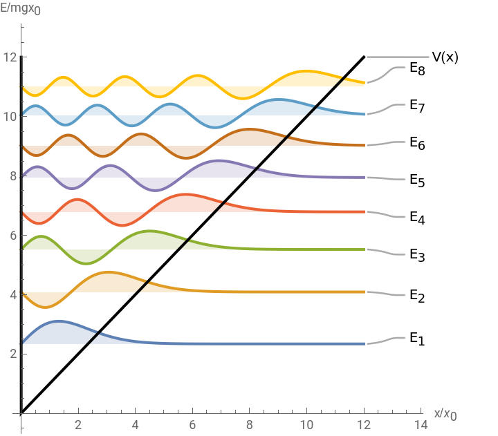
Plot eigenstates:
In[]:=
Show[Plot[Evaluate@Table[-AiryAiZero[n]+ps[n],{n,8}],{z,0,12},PlotRange->All,Filling->Table[n->-AiryAiZero[n],{n,8}],PlotLabelsTable[Subscript["E",ToString[n]],{n,8}],AxesLabel->{"x/","E/"}],Plot[If[x<=0,100,x],{x,-10^-3,13},PlotStyle->Black,PlotLabels->"V(x)",ExclusionsNone,PlotRange->{0,12}],AxesOrigin->{0,0},AspectRatio->1]
x
0
mgx
0
Out[]=
Time Evolution and Bouncing
Time Evolution and Bouncing
Define a Gaussian wave packet:
In[]:=
gaus=Exp[-(x-(x0=10))^2];=NIntegrate[gaus^2,{x,0,∞}];gaus=gaus
;Find the Gaussian in terms of the first 100 eigenstates:
In[]:=
coeff=TableNIntegrate[AiryAi[x+AiryAiZero[n]]gaus,{x,0,∞}],{n,100}//N//Quiet;
1
Abs[AiryAiPrime[AiryAiZero[n]]]
Get the maximum 10 terms with largest coefficients:
In[]:=
points=ReverseSortBy[Table[{i,coeff[[i]]},{i,Length[coeff]}],Abs@*Last][[;;10]];
Approximate the Gaussian with only those 10 terms and normalize it:
In[]:=
ψi=#[[2]]&/@points//Total;2=NIntegrate[ψi^2,{x,0,∞}];ψi=ψi
AiryAi[x+AiryAiZero[#[[1]]]]
Abs[AiryAiPrime[AiryAiZero[#[[1]]]]]
2
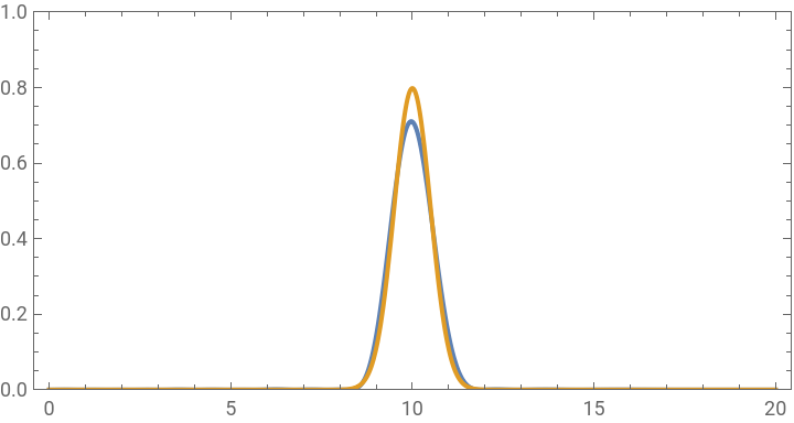
;Plot the approximated wavefunction and the original one for comparison:
In[]:=
Plot[{Abs[ψi]^2,Abs[gaus]^2},{x,0,20},PlotRange->{0,1},PlotLegends->{"Approximation","Original"},AspectRatio->1/2,Frame->True]
Out[]=


Overlap of approximated state with the expected Gaussian:
In[]:=
NIntegrate[ψigaus,{x,0,∞}]
Out[]=
0.995704
Time evolution:
In[]:=
ClearAll[ϕ];ϕ[t_]=Exp[AiryAiZero[#[[1]]]t]#[[2]]&/@points//Total;
AiryAi[x+AiryAiZero[#[[1]]]]
Abs[AiryAiPrime[AiryAiZero[#[[1]]]]]
Visualize the wavefunction:
In[]:=
Plot3D[Abs@ϕ[t],{t,0,10},{x,0,15},PlotRange->All,PlotPoints->50,ColorFunction->"Rainbow",AxesLabel->{"time","position","Abs[]"}]
ψ
t
Out[]=

Make a density plot:
In[]:=
DensityPlotAbs@ϕ[t],{t,0,10},{x,0,15},PlotRange->All,PlotPoints->100,AspectRatio->14,ImageSize->Large,ColorFunction->(ColorData["Rainbow"][]&),FrameLabel->{"time","Abs[]"}
1/2
#
ψ
t
Make an interactive animation of wavefunction evolution:
Acknowledgment
Acknowledgment
This notebook was developed by the Academic Innovation Team at Wolfram Research as part of our initiative to commemorate the International Quantum Year 2025. Our aim is to celebrate this milestone by offering engaging and innovative features that highlight the fascinating concepts and phenomena within quantum theory.
You can contact us at academicinnovation AT wolfram.com
You can contact us at academicinnovation AT wolfram.com
CITE THIS NOTEBOOK
CITE THIS NOTEBOOK
Quantum bouncer: 1-dimensional dynamical behavior
by Mohammad Bahrami
Wolfram Community, STAFF PICKS, December 12, 2024
https://community.wolfram.com/groups/-/m/t/3338419
by Mohammad Bahrami
Wolfram Community, STAFF PICKS, December 12, 2024
https://community.wolfram.com/groups/-/m/t/3338419