Cascade Control of a Water Tank Heating Process
Authors: Housam Binous and Ahmed Bellagi
Cascade Control of a Water Tank Heating Process
Authors: Housam Binous and Ahmed Bellagi
Authors: Housam Binous and Ahmed Bellagi
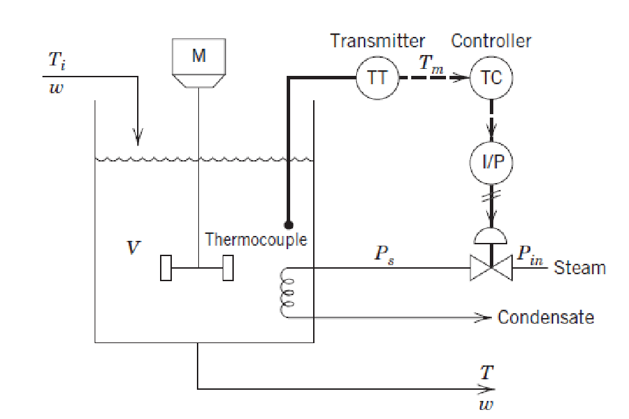
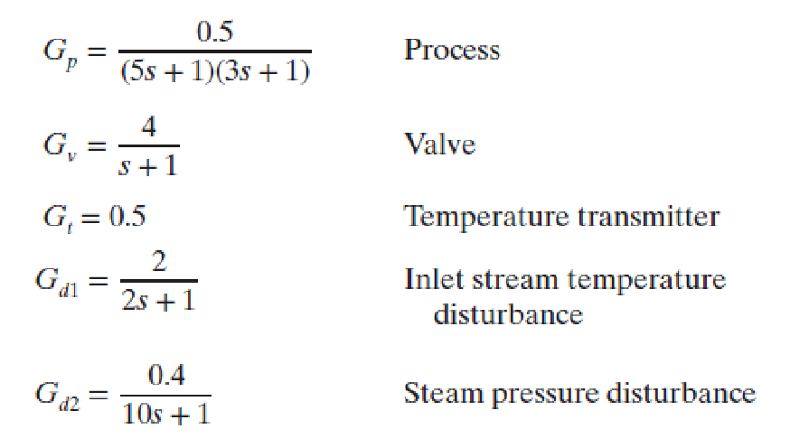
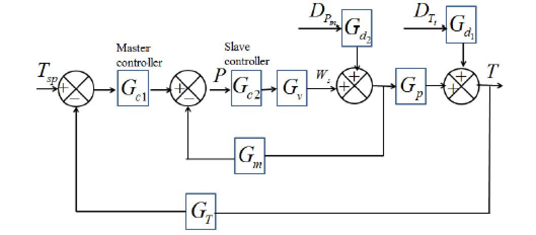
A water tank heating process is shown in the Figure below :We control the outlet temperature at a desired set point Tsp by manipulating the steam pressure Ps of steam sent to the tank heat exchanger. The steam delivery pressure Pin is subject to variations that affect Ps. Disturbances in the inlet stream temperature Ti are the primary disturbance to the process.The transfer functions of the system are :The block diagram corresponding to the system under consideration is given below :When one sets Gm=0 and Gc2=1 he recovers the classical feedback control configuration where: (a) Assuming that a PI controller with τI = 0.2 min is used, we find the ultimate gain for the standard single control loop configuration.(b) Now, we consdier a cascade control strategy, which is implemented to handle variations in upstream steam pressure or Pin. We take Gm = 0.4. The cascade controller closed-loop response is compared to that of the standard PI controller (Kc1 = 2 and τI1 = 5) for a unit step disturbance in steam pressure. For the cascade controller, we adopt: a PI controller for the master loopwith Kc1 = 2, τI1 = 5 and a P-only controller for the slave controller with Kc2 = 2.Reference :[1] D. E. Seborg, T. F. Edgar, D. A. Mellichamp, and F. J. Doyle III, Process Dynamics and Control, 4th ed., New York: Wiley, 2017.

Ultimate gain for the PI Controller of the standard control loop configuration is equal to 0.0778.
In[]:=
Gv=4/(s+1);Gp=0.5/(5s+1)/(3s+1);Gd2=0.4/(10s+1);Gt=0.5;Gd1=2/(2s+1);
In[]:=
tauI1=0.2;
In[]:=
Gc1=Kcu1(1+1/tauI1/s);
In[]:=
1+Gc1GvGpGt//Factor
Out[]=
0.0666667(5.Kcu1+1.s+1.Kcu1s+9.+23.+15.)
2
s
3
s
4
s
s(0.2+1.s)(0.333333+1.s)(1.+1.s)
In[]:=
sol=NSolve[5.Kcu1+1.s+1.Kcu1s+9.s^2+23.s^3+15.s^40,s];
In[]:=
s1=s/.sol[[3]];
In[]:=
solu=FindRoot[Re[s1]0,{Kcu1,0.1}]
Out[]=
{Kcu10.077759}
In[]:=
sol/.solu//Chop
Out[]=
{{s-0.952776},{s-0.580557},{s0.-0.21647},{s0.+0.21647}}
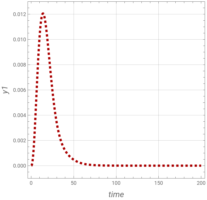
A comparison of D2 unit step responses with (dashed red) and without (blue) cascade control.
Clearly, we demonstrate that the cascade control system is clearly superior to a conventional PI controller for a secondary loop disturbance
Clearly, we demonstrate that the cascade control system is clearly superior to a conventional PI controller for a secondary loop disturbance
In[]:=
Gm=0.4;
In[]:=
Kc1=2;tauI1=5.;
In[]:=
Gc1=Kc1(1+1/tauI1/s)
Out[]=
21+
0.2
s
In[]:=
Gc2=Kc2;Kc2=2;
In[]:=
Ycascade=1/sGpGd2/(1+Gc2GvGm+Gc1Gc2GvGpGt)//Factor
Out[]=
0.00133333(1.+1.s)
(0.1+1.s)(0.2+1.s)(4.21629+1.s)(0.0632468+0.317045s+1.)
2
s
In[]:=
ycascade=InverseLaplaceTransform[Ycascade,s,t]
Out[]=
0.00133333(-0.0117882-50.+52.6316-(1.3099-13.3219)((-0.980849+0.19477)+(1.+0.)))
-4.21629t
-0.2t
-0.1t
(-0.158523-0.195237)t
(0.+0.390474)t
In[]:=
YPIConventional=1/sGd2Gp/(1+Gc1GvGpGt)//Factor
Out[]=
0.00133333(1.+1.s)
(0.1+1.s)(0.2+1.s)(1.14382+1.s)(0.116568+0.189509s+1.)
2
s
In[]:=
yPIConventional=InverseLaplaceTransform[YPIConventional,s,t]
Out[]=
0.00133333(-0.120836-71.4286+80.1187-(4.28464-11.012)((-0.73703+0.67586)+(1.+0.)))
-1.14382t
-0.2t
-0.1t
(-0.0947546-0.328009)t
(0.+0.656017)t
In[]:=
p1=Plot[ycascade,{t,0,200},FrameTrue,GridLinesAutomatic,AspectRatio1,FrameLabel{Style["time",14,Italic],Style["y1",14,Italic]},PlotRange{All,{-0.001,0.013}},PlotStyle{Thickness[0.0125],Dashed,Darker@Red}]
Out[]=
In[]:=
p2=Plot[yPIConventional,{t,0,200},FrameTrue,GridLinesAutomatic,AspectRatio1,FrameLabel{Style["time",14,Italic],Style["y1",14,Italic]},PlotRange{All,{-0.005,0.035}},PlotStyle{Thickness[0.0125],Dashed,Darker@Blue}]
A comparison between our calculations and their counterparts shown in yellow and obtained using SIMULINK.