Calculating the cumulative incidence is easy for a simple SIR model - the decline in susceptibility shows us how many people have become infected . First, notice that for every incident case, the value of goes down by 1. So to calculate the total incidence in a given time interval, we just need to calculate the amount by which susceptiblity has fallen in that same time period . This is the approach in the following example .
S
Given parameters
γ=0.2;β=0.4;tMax=100;n=1000;
Define the force of infection (λ)
λ[t_]:=βi[t]/n;
Define the system of differential equations
eqns={s'[t]==-λ[t]s[t],i'[t]==λ[t]s[t]-γi[t],r'[t]==γi[t],s[0]==1000,i[0]==1,r[0]==0};
Solve the system
sol=NDSolve[eqns,{s,i,r},{t,0,tMax}][[1]];
In[]:=
case0=s[0]/.sol
Out[]=
1000.
In[]:=
case101=s[100]/.sol
Out[]=
202.615
In[]:=
Difference=case0-case101
Out[]=
797.385
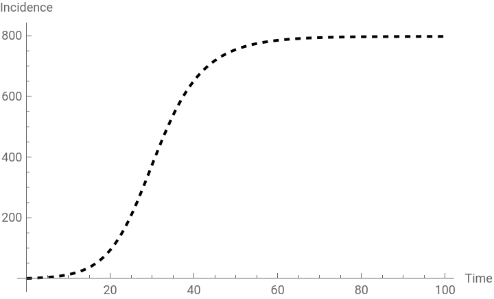
From this,we can see that a total of 797 cases occurred during the epidemic . This number is the cumulative incidence .
A flexible approach
A flexible approach
For the simple SIR model, the previous approach is sufficient, but if we want to calculate incidence in more complex models, the following code will help us
Cumulative incidence function
inc[tmax_]:=NIntegrate[λ[t]s[t]/.sol,{t,0,tmax}];
In[]:=
cump=Plot[inc[u],{u,0,100},AxesLabel->{"Time","Incidence"},PlotLegends->{"cumulative incidence"},PlotStyle->{Black,Dashed}]
Out[]=

In[]:=
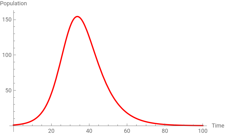
p=Plot[Evaluate[{i[t]}/.sol],{t,0,tMax},PlotLegends->{"Infected"},AxesLabel->{"Time","Population"},PlotStyle->{Red}]
Out[]=

In[]:=
Show[p,cump,PlotRange->All]
Out[]=
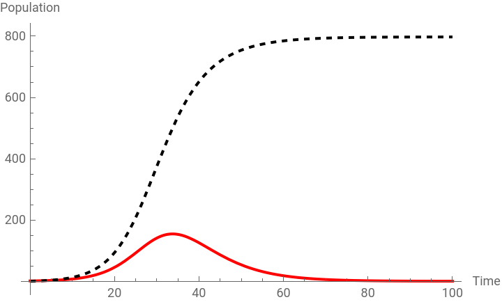
The plot shows us that at the peak of the epidemic on day 34, 154 people were infected . By that time, a total of 506 people had been infected . By the end of the epidemic, around 75 days after the start of the simulation, nearly 800 people had been infected in total .
Create a table with S, I, R, and inc values
timeValues=Range[0,tMax,1];table=Table[{t,s[t]/.sol,i[t]/.sol,r[t]/.sol,inc[t]},{t,timeValues}];
Display the combined table with appropriate headers
Grid[Prepend[table,{"Time","Susceptible","Infected","Recovered","Cumulative Incidence"}],Dividers->All]
Out[]=
Time | Susceptible | Infected | Recovered | Cumulative Incidence |
0 | 1000. | 1. | 0. | 0. |
1 | 999.557 | 1.2213 | 0.221396 | 0.442694 |
2 | 999.017 | 1.49128 | 0.491761 | 0.983038 |
3 | 998.358 | 1.8205 | 0.821852 | 1.64235 |
4 | 997.553 | 2.22176 | 1.22476 | 2.44652 |
5 | 996.573 | 2.71049 | 1.71638 | 3.42688 |
6 | 995.379 | 3.30531 | 2.31602 | 4.62133 |
7 | 993.924 | 4.02852 | 3.04705 | 6.07558 |
8 | 992.155 | 4.90682 | 3.93775 | 7.84458 |
9 | 990.006 | 5.97195 | 5.02222 | 9.99417 |
10 | 987.397 | 7.26139 | 6.34148 | 12.6029 |
11 | 984.236 | 8.81908 | 7.94464 | 15.7637 |
12 | 980.414 | 10.696 | 9.89037 | 19.5864 |
13 | 975.801 | 12.9506 | 12.2482 | 24.1988 |
14 | 970.251 | 15.6487 | 15.1002 | 29.7489 |
15 | 963.595 | 18.8629 | 18.5421 | 36.405 |
16 | 955.644 | 22.6711 | 22.6849 | 44.356 |
17 | 946.191 | 27.1537 | 27.6555 | 53.8091 |
18 | 935.015 | 32.3889 | 33.5966 | 64.9854 |
19 | 921.888 | 38.4463 | 40.6659 | 78.1122 |
20 | 906.588 | 45.3783 | 49.0335 | 93.4118 |
21 | 888.914 | 53.2085 | 58.8772 | 111.086 |
22 | 868.705 | 61.9191 | 70.3757 | 131.295 |
23 | 845.863 | 71.438 | 83.6989 | 154.137 |
24 | 820.377 | 81.6274 | 98.9957 | 179.623 |
25 | 792.343 | 92.2767 | 116.381 | 207.657 |
26 | 761.979 | 103.103 | 135.918 | 238.021 |
27 | 729.627 | 113.762 | 157.611 | 270.373 |
28 | 695.745 | 123.869 | 181.386 | 304.256 |
29 | 660.875 | 133.03 | 207.095 | 339.125 |
30 | 625.615 | 140.875 | 234.51 | 374.385 |
31 | 590.566 | 147.097 | 263.337 | 409.434 |
32 | 556.297 | 151.476 | 293.226 | 443.703 |
33 | 523.304 | 153.9 | 323.797 | 476.696 |
34 | 491.984 | 154.361 | 354.655 | 508.017 |
35 | 462.627 | 152.956 | 385.417 | 537.373 |
36 | 435.418 | 149.858 | 415.724 | 564.582 |
37 | 410.44 | 145.297 | 445.262 | 589.56 |
38 | 387.699 | 139.538 | 473.763 | 612.301 |
39 | 367.133 | 132.851 | 501.016 | 632.867 |
40 | 348.639 | 125.502 | 526.86 | 651.361 |
41 | 332.081 | 117.731 | 551.188 | 667.919 |
42 | 317.31 | 109.752 | 573.938 | 682.69 |
43 | 304.168 | 101.745 | 595.087 | 695.832 |
44 | 292.501 | 93.8552 | 614.644 | 707.499 |
45 | 282.158 | 86.1977 | 632.645 | 717.842 |
46 | 272.999 | 78.8571 | 649.144 | 727.001 |
47 | 264.894 | 71.8933 | 664.213 | 735.106 |
48 | 257.726 | 65.3447 | 677.929 | 742.274 |
49 | 251.388 | 59.2327 | 690.38 | 748.612 |
50 | 245.784 | 53.5644 | 701.652 | 754.217 |
51 | 240.829 | 48.3365 | 711.835 | 759.171 |
52 | 236.447 | 43.5376 | 721.015 | 763.553 |
53 | 232.572 | 39.1505 | 729.277 | 767.428 |
54 | 229.144 | 35.1541 | 736.702 | 770.856 |
55 | 226.111 | 31.525 | 743.364 | 773.889 |
56 | 223.427 | 28.2382 | 749.334 | 776.573 |
57 | 221.051 | 25.2686 | 754.68 | 778.949 |
58 | 218.948 | 22.5911 | 759.461 | 781.052 |
59 | 217.085 | 20.1812 | 763.734 | 782.915 |
60 | 215.434 | 18.0158 | 767.55 | 784.566 |
61 | 213.972 | 16.0728 | 770.955 | 786.028 |
62 | 212.676 | 14.3314 | 773.993 | 787.324 |
63 | 211.528 | 12.7724 | 776.7 | 788.472 |
64 | 210.509 | 11.3781 | 779.113 | 789.491 |
65 | 209.607 | 10.1321 | 781.261 | 790.393 |
66 | 208.806 | 9.01949 | 783.174 | 791.194 |
67 | 208.096 | 8.02664 | 784.877 | 791.904 |
68 | 207.467 | 7.14116 | 786.392 | 792.533 |
69 | 206.908 | 6.35187 | 787.74 | 793.092 |
70 | 206.413 | 5.64862 | 788.939 | 793.587 |
71 | 205.973 | 5.02229 | 790.004 | 794.027 |
72 | 205.583 | 4.46468 | 790.952 | 794.417 |
73 | 205.237 | 3.96838 | 791.794 | 794.763 |
74 | 204.93 | 3.5268 | 792.543 | 795.07 |
75 | 204.658 | 3.13399 | 793.208 | 795.342 |
76 | 204.416 | 2.78465 | 793.8 | 795.584 |
77 | 204.201 | 2.47402 | 794.325 | 795.799 |
78 | 204.011 | 2.19786 | 794.791 | 795.989 |
79 | 203.842 | 1.95239 | 795.206 | 796.158 |
80 | 203.692 | 1.73423 | 795.574 | 796.308 |
81 | 203.558 | 1.54035 | 795.901 | 796.442 |
82 | 203.44 | 1.36808 | 796.192 | 796.56 |
83 | 203.335 | 1.21502 | 796.45 | 796.665 |
84 | 203.242 | 1.07905 | 796.679 | 796.758 |
85 | 203.159 | 0.958254 | 796.882 | 796.841 |
86 | 203.086 | 0.850958 | 797.063 | 796.914 |
87 | 203.021 | 0.755654 | 797.224 | 796.979 |
88 | 202.963 | 0.671006 | 797.366 | 797.037 |
89 | 202.912 | 0.59583 | 797.493 | 797.089 |
90 | 202.866 | 0.529064 | 797.605 | 797.134 |
91 | 202.825 | 0.469772 | 797.705 | 797.175 |
92 | 202.79 | 0.417119 | 797.793 | 797.211 |
93 | 202.758 | 0.370362 | 797.872 | 797.242 |
94 | 202.729 | 0.328842 | 797.942 | 797.271 |
95 | 202.704 | 0.291974 | 798.004 | 797.296 |
96 | 202.682 | 0.259236 | 798.059 | 797.318 |
97 | 202.662 | 0.230168 | 798.108 | 797.338 |
98 | 202.644 | 0.204358 | 798.151 | 797.356 |
99 | 202.629 | 0.18144 | 798.19 | 797.371 |
100 | 202.615 | 0.161092 | 798.224 | 797.385 |
◼
From the cumulative incidence at each timestep, we can easily calculate how many infections occurred between any 2 timesteps, as follows:
We calculate the difference between the cumulative incidence at each given timestep minus the cumulative incidence at the preceding timestep . Adding a 0 as the first value, the incident_infections vector shows you how many infections have occurred in the intervals between each timestep .
Calculate the difference in cumulative incidence
Create tables for S, I, R, Cumulative Incidence, and Incident Infections
Display the combined table with appropriate headers
We might also want to know how many new cases occurred during a specific time, such as after the peak of the epidemic, e . g . between day 40 and 75.
Difference of cumulative incidence at day 75 and cumulative incidence at day 40 :
Calculate cumulative incidence at day 40 and 75
Calculate the difference of cumulative incidence at day 75 and day 40
Display the result
Even after the peak of the epidemic was already reached, 144 new infections still occurred .
CITE THIS NOTEBOOK
CITE THIS NOTEBOOK
Calculating incidence in a deterministic SIR model
by Athanasios Paraskevopoulos
Wolfram Community, STAFF PICKS, September 6, 2023
https://community.wolfram.com/groups/-/m/t/3007127
by Athanasios Paraskevopoulos
Wolfram Community, STAFF PICKS, September 6, 2023
https://community.wolfram.com/groups/-/m/t/3007127