ABSTRACT (original article): The present paper describes how to apply the Chebyshev orthogonal collocation technique to solve steady-state and unsteady-steady two-dimensional problems. All problems are solved using one single computer algebra, Mathematica©. The problems include: (1) steady-state heat transfer in a rectangular bar, (2) steady-state flow in a rectangular duct, (2) steady-state heat transfer in a cooling cylindrical pin fin, (4) steady-state heat conduction in an annulus, (5) unsteady-state heat transfer in a rectangular bar, and finally (6) unsteady-state diffusion reaction system. Whenever possible the results obtained with orthogonal collocation are compared to the analytical solution in order to validate the applied numerical technique. CITATION (original article): Binous, H., Kaddeche, S., & Bellagi, A. (2015). Solving two-dimensional chemical engineering problems using the chebyshev orthogonal collocation technique. In Computer Applications in Engineering Education (Vol. 24, Issue 1, pp. 144–155). Wiley. DOI: https://doi.org/10.1002/cae.21680
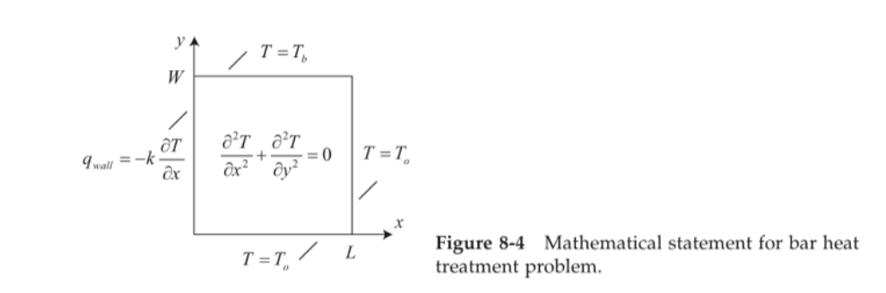
Consider a bar with a rectangular cross section subject to both temperature and heat flux boundary conditions.The governing equation and boundary conditions in dimensionless form are:θ+θ=0, with and ,=- (continuity of heat flux at the boundary), (constant temperature at the boundary), (same constant temperature at the boundary), and (different constant temperature at the boundary),with , , and .
2
∂
∂
2
x
2
∂
∂
2
y
0≤x≤L
0≤y≤W
∂θ
∂x
x=0
q
w
k
x=0
θ(x=L)=0
x=L
θ(y=0)=0
y=0
θ(y=W)=
θ
b
y=W
W=1
L=1
k=0.01
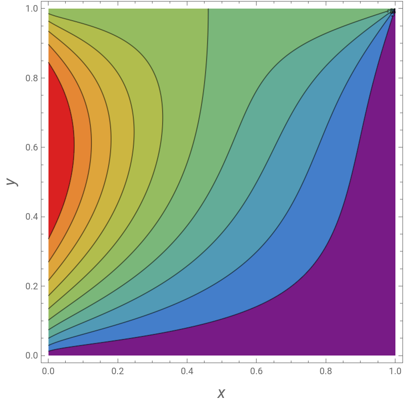
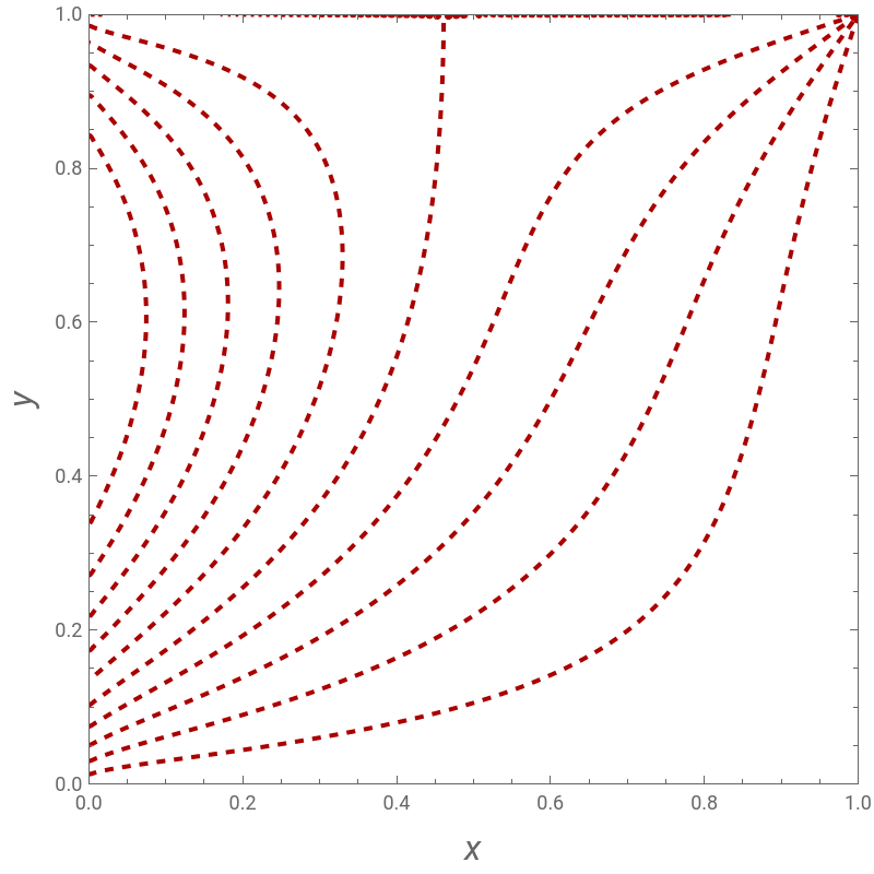
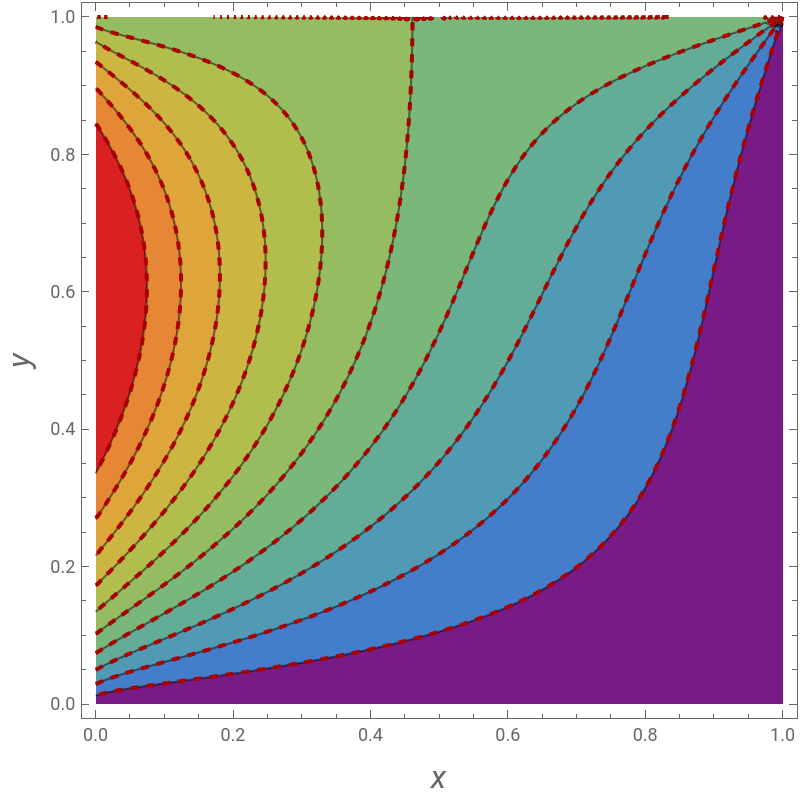
The Chebyshev orthogonal collocation method implemented in Mathematica with =41 collocation points (see Ref. 1) gives the temperature distribution in the bar for =1 and =20.The analytical solution of the differential equation obtained using the separation of variables technique [2] is given by:,where =.As shown below, we find excellent agreement between our numerical solution and the analytical solution.
N
p
q
w
θ
b
θ=sin( L)sinh( y)+1-cos( x)
∞
∑
n=0
2
L
λ
n
θ
b
λ
n
λ
n
sinh( W)
λ
n
q
w
k
λ
n
sinh( y)+sinh( (W-y))
λ
n
λ
n
sinh( W)
λ
n
λ
n
λ
n
(2 n+1) π
2L
Parameters of the problem reproduced from Ref . 2.
In[]:=
L=1;W=1;k=0.01;qwall=1;thetab=20;
Numerical solution based on Orthogonal Collocation and the Gauss - Lobatto nodes
Derivative Matrices constructed using 41 Gauss - Lobatto collocation points
In[]:=
Np=40;Ds=Table[d[i,j],{i,0,Np},{j,0,Np}];d[0,0]=(2Np^2+1)/6//N;d[Np,Np]=-(2Np^2+1)/6//N;d[i_,i_]:=-y[i]/(2(1-y[i]^2));y[i_]:=Cos[iPi/Np]//N;d[j_,k_]:=If[j≠k,c[j](-1)^(j+k)/(c[k](y[j]-y[k]))];c[i_]:=If[i0||iNp,2,1];Dsq=Ds.Ds;
In[]:=
L2=(2/W)^2KroneckerProduct[Dsq,IdentityMatrix[Np+1]]+(2/L)^2KroneckerProduct[IdentityMatrix[Np+1],Dsq];Lbc=(2/L)KroneckerProduct[IdentityMatrix[Np+1],Ds];
Governing equations
In[]:=
x=Table[L/2(1+y[i]),{i,Np,0,-1}];
In[]:=
U=Table[u[i+(j-1)(Np+1)],{j,1,Np+1},{i,1,Np+1}]//Flatten;
In[]:=
Eq[i_]:=L2[[i]].U0;
In[]:=
bc=Table[Lbc[[1+(j-1)(Np+1)]].Uqwall/k,{j,2,Np}];
In[]:=
sys=Join[{Table[u[i]0,{i,1,Np+1}],bc,Table[u[Np+1+(j-1)(Np+1)]0,{j,2,Np}],Table[u[i+Np(Np+1)]thetab,{i,1,Np+1}],Table[Eq[i+(j-1)(Np+1)],{j,2,Np},{i,2,Np}]}]//Flatten;
In[]:=
initguess=Flatten[Table[{u[i+(j-1)(Np+1)],20},{j,1,Np+1},{i,1,Np+1}],1];
Solution using FindRoot
In[]:=
sol=Quiet@FindRoot[sys,initguess];
Contour plot of the solution
In[]:=
a=Flatten[Table[{x[[i]],x[[j]],u[i+(j-1)(Np+1)]/.sol},{j,1,Np+1},{i,1,Np+1}],1];f=Interpolation[a,InterpolationOrder3];
In[]:=
p1=ContourPlot[f[x1,y1],{x1,0,L},{y1,0,W},ContoursTable[4i,{i,1,10,1}],PlotPoints100,ImageSize{400,400},FrameLabel{Style["x",Italic,16],Style["y",Italic,16]},PlotLegendsAutomatic,ColorFunction"Rainbow"]
Out[]=

Analytical solution
In[]:=
θ[x_,y_]:=Sum+1-Cos[λ[n] x],{n,0,200}
2
L λ[n]
thetabSin[λ[n] L]Sinh[λ[n] y]
Sinh[λ[n] W]
qwall
kλ[n]
Sinh[λ[n] y]+Sinh[λ[n] (W-y)]
Sinh[λ[n] W]
In[]:=
λ[n_]:=
(2n+1)Pi
2L
In[]:=
p2=ContourPlot[θ[x1,y1],{x1,0,L},{y1,0,W},ContoursTable[4i,{i,1,10,1}],PlotPoints100,ImageSize{400,400},FrameLabel{Style["x",Italic,16],Style["y",Italic,16]},ContourStyle->Table[{Dashed,Thick,Darker@Red},{i,1,10,1}],ContourShading->None,PlotRange->{{0,1},{0,1}}]
Out[]=
Analytical + Numerical solutions superimposed on the same plot
In[]:=
Show[p1,p2,PlotRange->{{0,1},{0,1}}]
Out[]=
References:
References:
◼
[1] H. Binous, S. Kaddeche and A. Bellagi, Solving two-dimensional chemical engineering problems using the chebyshev orthogonal collocation technique, Computer Applications in Engineering Education, 24(1), pp. 144-155, 2016.
◼
[2] T. Bennett, Transport by Advection and Diffusion, New York: Wiley, 2012.
CITE THIS NOTEBOOK
CITE THIS NOTEBOOK
Heat transfer in a bar with rectangular cross section
by Housam Binous and Ahmed Bellagi
Wolfram Community, STAFF PICKS, March 23, 2024
https://community.wolfram.com/groups/-/m/t/3146178
by Housam Binous and Ahmed Bellagi
Wolfram Community, STAFF PICKS, March 23, 2024
https://community.wolfram.com/groups/-/m/t/3146178