ABSTRACT (original article): In the present paper, we present the solution of four problems drawn from the chemical and biochemical engineering field of study. These problems illustrate various important aspects of nonlinear dynamics such as limit cycles, quasi-periodic and chaotic behaviors, time series and phase portraits, power spectra, the time-delay reconstruction diagrams, Hopf bifurcation, bifurcation diagrams, steady state multiplicity… Among a large number of examples, we have selected the following case studies because they illustrate the basic nonlinear dynamics concepts listed previously: (i) The glycolytic oscillator model, first suggested by Sel’kov in 1968 in order to elucidate the mechanism that living cells use to obtain energy from sugar breakdown; (ii) The Oregonator model derived by Field, Körös, and Noyes in the early 1970s, which elucidates the famous oscillatory behavior observed in the Belousov–Zhabotinsky reaction; (iii) The steady state multiplicity in a biochemical reactor for both the Monod and substrate inhibition kinetics; and (iv) The three-variable autocatalator, first proposed by Peng, Scott, and Showalter in 1990. Finally, we conclude this paper by sharing our experience teaching this subject to graduate students at King Fahd University of Petroleum & Minerals (KFUPM). CITATION (original article): Binous, H., & Bellagi, A. (2018). Introducing nonlinear dynamics to chemical and biochemical engineering graduate students using MATHEMATICA©. Computer Applications in Engineering Education, 27(1), 217–235. https://doi.org/10.1002/cae.22070
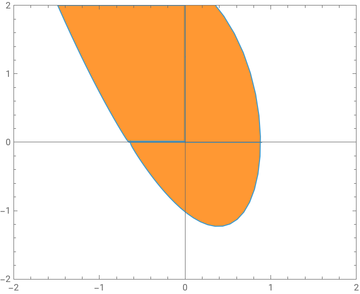
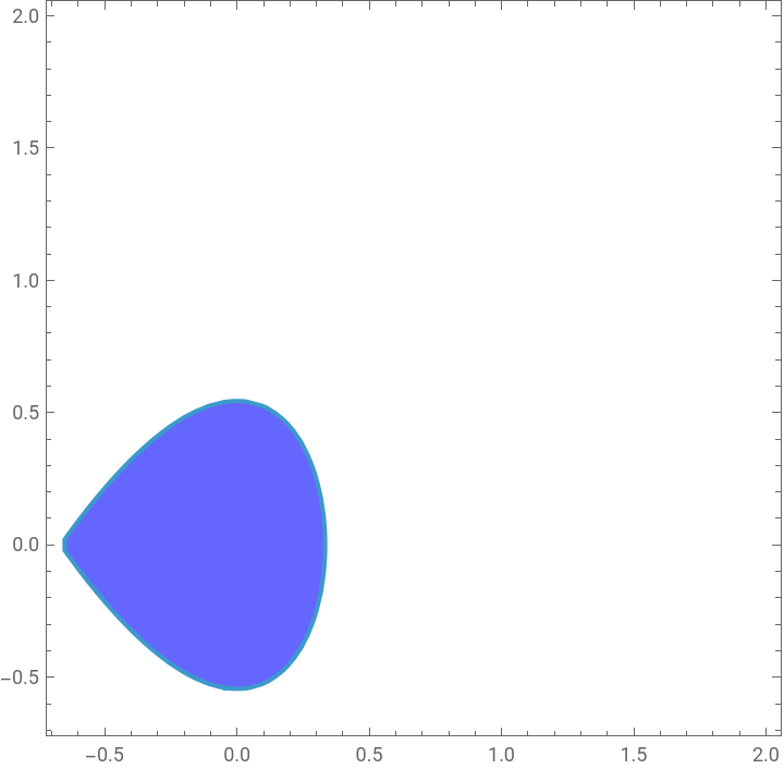
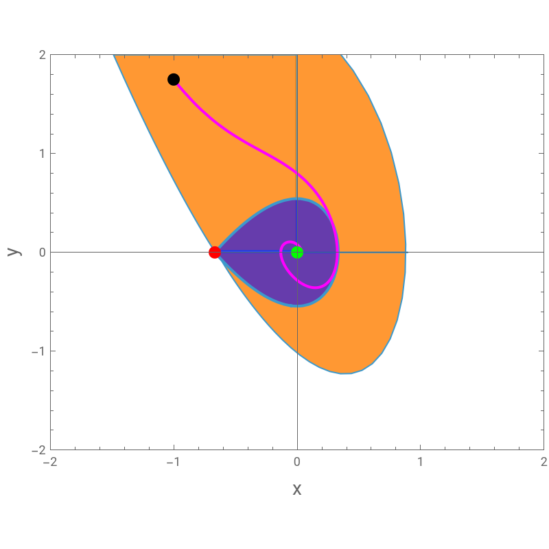
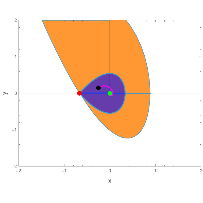
Consider the two-dimensional autonomous dynamical system:=y,=-2bx-3-ay.There are two steady states, =(0,0) and =(-2b/3,0), shown by the green and red points. Restricting the parameters to and , we compute numerically and plot the region of asymptotic stability (RAS), shown in orange. The blue region is also an RAS for . This region is obtained using Lyapunov’s direct method and the Lyapunov function . The blue region cannot contain because it is an unstable steady state. defines a closed curve containing the origin if is a positive constant. The largest such region can be obtained by having at its frontier, or if b=1 we get S2={-0.666,0} and K=0.148.
x
t
y
t
2
x
S
1
S
2
a=1
b=1
S
1
V(x,y)=b++2
2
x
3
x
2
y
S
2
V=K
K
S
2
K=4/27
3
b
“Note that the RAS of the origin, as determined by the Liapunov function, is smaller than the actual RAS determined numerically. In fact, this occurs frequently and is a limitation of the method. However, it should also be noted that the smaller RAS is obtained analytically with relatively little effort.” (Ref. 1)
“The region of asymptotic stability is often used to describe the set of all states where the system can remain stable, while the basin of attraction is used to describe the set of all states where the system can converge to a particular equilibrium point.” (source internet)
Kindly check Ref. 2 for more on nonlinear dynamics in the chemical and biochemical engineering curricula.
In[]:=
odes={x'[t]y[t],y'[t]-2b1x[t]-3x[t]^2-a1y[t]};(*thetwo-dimensionalautonomousdynamicalsystem*)a1=1;b1=1;sol[a_?NumericQ]:=NDSolve[{odes,x[0]a,y[0]2.475},{x[t],y[t]},{t,0,tmax}];sol1[a_,b_]:=NDSolve[{odes,x[0]a,y[0]b},{x[t],y[t]},{t,0,tmax}];
In[]:=
(*numericalcomputationtheregionofasymptoticstability-shownbelowinorange*)tmax=4;eq[a_?NumericQ]:=(((x[t]/.sol[a][[1]])/.t4)+2b1/3);s1=FindRoot[eq[e]0,{e,0.1,0.6}];c1=ParametricPlot[Evaluate[{x[t],vy[t]}/.sol1[e/.s1,2.45]],{t,0,4},{v,0,1},PlotStyleDirective[Orange,Opacity[0.8]],PlotRange{{-2,2},{-2,2}},AspectRatio0.8,FrameTrue,GridLinesNone,MeshStyleNone];tmax=2.45;sol[a_?NumericQ]:=NDSolve[{odes,x[0]a,y[0]2.0},{x[t],y[t]},{t,0,tmax}];eq[a_?NumericQ]:=(((x[t]/.sol[a][[1]])/.ttmax)+2b1/3);s1=FindRoot[eq[e]0,{e,-1.5}];c2=ParametricPlot[Evaluate[{vx[t],y[t]}/.sol1[e/.s1,2.0]],{t,0,tmax},{v,0,1},PlotStyleDirective[Orange,Opacity[0.8]],PlotRange{{-2,2},{-2,2}},AspectRatio0.8,FrameTrue,GridLinesNone,MeshStyleNone];
In[]:=
Show[c1,c2]
Out[]=
In[]:=
(*computingtheRASfor-shownbelowinblue*)c3=RegionPlot[b1x^2+x^3+y^2/2-4b1^3/27≤0,{x,-2b1/3,2},{y,-2b1/3,2},PlotStyle{Opacity[0.6],Blue}];
S
1
In[]:=
Show[c3]
Out[]=
In[]:=
Min[10,Quiet@First@First[sol1[1,1][[2]]]]
Out[]=
Min10,x[t]InterpolatingFunction[t],y[t]InterpolatingFunction[t]


In[]:=
sol1[a_,b_]:=Reap[NDSolve[{odes,x[0]a,y[0]b,WhenEvent[Abs[y[t]]>5,{Sow[t],"StopIntegration"}]},{x[t],y[t]},{t,0,10}]];plt1[a_,b_]:=ParametricPlot[Evaluate[{x[t],y[t]}/.sol1[a,b][[1]]],{t,0,Min[10,Quiet@First@First[sol1[a,b][[2]]]]},PlotStyle{Magenta,Thick}]plt2[a0_,b0_]:=Show[c1,c2,c3,plt1[a0,b0],Graphics[{PointSize[0.025],Black,Point[{a0,b0}],Green,PointSize[0.025],Point[{0,0}],Red,Point[{-2b1/3,0}]}],ImageSize400{1,1},FrameLabel->{Style["x",14],Style["y",14]}](*IC={a0,b0}*)
All trajectories originating at an Initial Condition chosen in this orange region end at the Subscript[S, 1]. Trajectories diverge otherwise.
In[]:=
plt2[-1,1.75](*convergingtrajectory*)
Out[]=
In[]:=
plt2[-0.25,0.15](*convergingtrajectory*)
Out[]=
References
References
◼
[1] A. Varma and M. Morbidelli, Mathematical Methods in Chemical Engineering, New York: Oxford University Press, 1997.
◼
[2] H. Binous and A. Bellagi, Introducing nonlinear dynamics to chemical and biochemical engineering graduate students using MATHEMATICA©, Computer Applications in Engineering Education, 27 (1), pp . 217 - 235, 2019. https://doi.org/10.1002/cae.22070
CITE THIS NOTEBOOK
CITE THIS NOTEBOOK
Asymptotic stability of dynamical system by Lyapunov's direct method
by Housam Binous and Ahmed Bellagi
Wolfram Community, STAFF PICKS, September 21, 2025
https://community.wolfram.com/groups/-/m/t/3548370
by Housam Binous and Ahmed Bellagi
Wolfram Community, STAFF PICKS, September 21, 2025
https://community.wolfram.com/groups/-/m/t/3548370