Simulation is one of the major computing challenges for experiments like Belle II that take large amounts of data. The full simulation process consists of a typically fast event generation step, where decay chains from the initially produced particles to stable final state particles are simulated. Then, a powerful selection discards a large fraction of background events. The fraction of retained simulated background events is quite low. Therefore significant computing resources are wasted to produce simulated background events that are then discarded. Thus, in this project, an attempt is made to train a model based on Graph Neural Network approach by setting up a filter after the event generation stage which allows only few decay chains to pass through it, thus saving a great amount of computer resources. There are 9 features assigned to each of the particles in the events, based on which a training set is prepared. A mother particle index is also generated for every event, that is used to create an adjacency graph for the neural network input training data. The output consist of a list of binary data, where a ‘1’ signifies passing of an event through the filter. Other than this, the project also aims to visualize various features of the particles in form of graphs and histograms.
Introduction
Introduction
The goal of this classification problem is to identify generated events from the Belle II simulation dataset, that pass a selection already before the expensive simulation and reconstruction and to visualize the various parameters associated with each particle in graphical form. The event datasets along with other information are available as numpy arrays in the Github repository: https://github.com/kahn-jms/belle-selective-mc-dataset
Importing the Datasets
Importing the Datasets
Handling the Datasets
Handling the Datasets
Visualization of the Data
Visualization of the Data
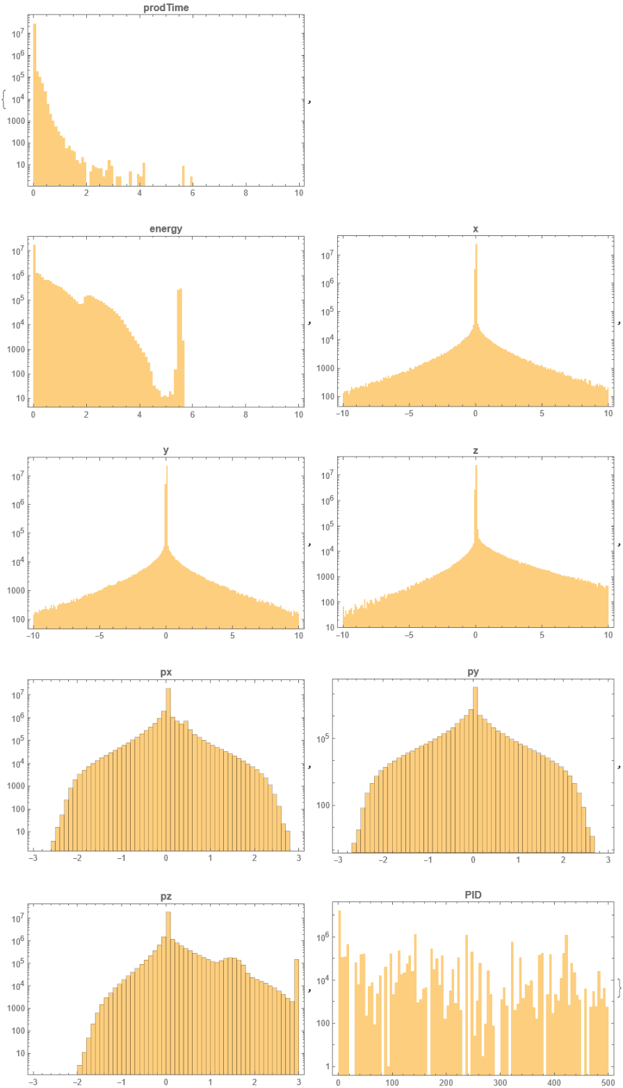
In order to visualize the 9 features of the Data, let us first create a label list and range list.
The label list is as follows:
In[]:=
Style[labels={"prodTime","energy","x","y","z","px","py","pz","PID"},Bold]labels//Length
The range list is as follows:
In[]:=
axisranges={{0,10,.1},{0,10,.1},{-10,10,.1},{-10,10,.1},{-10,10,.1},{-3,3,.1},{-3,3,.1},{-3,3,.1},{0,500,5}};axisranges//Length
Now, we generate a dataset with keys as labels above and values as corresponding numerical values.
In[]:=
dsLabeled=AssociationThread[labels,Transpose@Flatten[dt,1]];
We can visualize the data in the form of Histograms for each of the Data features.
In[]:=
Table[Histogram[dsLabeled[[i]],axisranges[[i]],ScalingFunctions"Log",ImageSizeMedium,PlotLabelStyle[labels[[i]],Bold],FrameTrue],{i,1,Length[labels]}]
Out[]=
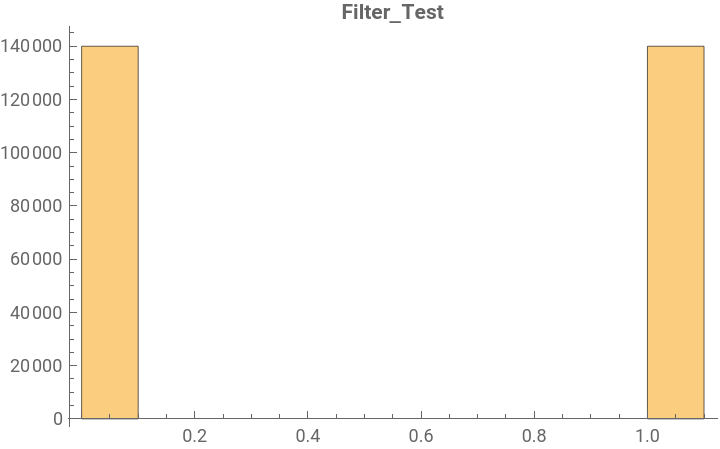
Similarly, the filter result data in binary can be visualized for all the events.
In[]:=
Histogram[dt4,{.1},PlotLabelStyle[Filter_Test,Bold]]
Out[]=
Classification Process
Classification Process
The Datasets in the original link also includes two extra datasets, which contains the information about mother particles in each of the event. Hence these datasets are 2-dimensional lists which contains 100 indices of mother particles for each of the event. For those events, where the particle numbers are less than 100, the elements have been padded with a -1 entry. This list is used to create the adjacency matrix for creating the graph of each event. The rules for creating the adjacency matrix in the original work were complicated to understand, hence I was not able to successfully generate the adjacency matrix. This matrix is always required to train a graph neural network model. Because, of the this issue, I took on a different approach for classification of the data: Fully Connected Network (FCN), which I am going to discuss about in the upcoming sub-section. Let me here present the approach that I was following to unsuccessfully generate the adjacency matrix.
For this, let us first import the dataset required for this task.
For this, let us first import the dataset required for this task.
In[]:=
dt2=ReadNumPyArray["C:/Users/Utkarsh/Downloads/Mathematica_Project/X_train_1.npy"];
The original work was implemented in python language, so I tried to use python as the external evaluator for this particular problem in hand. For this, I had to successfully integrate python evaluator in Wolfram Mathematica.
In[]:=
RegisterExternalEvaluator["Python","C:\\Users\\Utkarsh\\AppData\\Local\\Programs\\Python\\Python38-32\\python.exe"]
Out[]=
554f220a-08fd-6279-05c7-9734f6dd5d73
In[]:=
FindExternalEvaluators["Python"]
Out[]=

The following code as taken from the original work and then modified according to our need did not execute as intended.
In[]:=
import numpy as np
dt3=np.load("C:\\Users\\Utkarsh\\Downloads\\Mathematica_Project\\X_train_1.npy")
def adjacency_matrix_from_mothers_np(mother_indices):
N = mother_indices.shape[1]
adj = np.eye(N + 1, dtype=np.int8)[mother_indices][:,:,:-1]
return adj
adjacency_matrix_from_mothers_np(dt3)
dt3=np.load("C:\\Users\\Utkarsh\\Downloads\\Mathematica_Project\\X_train_1.npy")
def adjacency_matrix_from_mothers_np(mother_indices):
N = mother_indices.shape[1]
adj = np.eye(N + 1, dtype=np.int8)[mother_indices][:,:,:-1]
return adj
adjacency_matrix_from_mothers_np(dt3)
Out[]=
Failure

Thus, next I implemented FCN for the problem in hand. The FCN layer layout is a bit straightforward compared to Graph Neural Network and does not require an adjacency matrix, as no graphical structure is required for the fed input.
Classification via FCN
Classification via FCN
The schematic representation of the FCN as presented in the original work can be seen from the following image( taken from the original work):
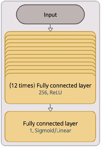
Based, on this schematic, a neural network model can be defined as follows:
Input and output variables are created by taking first 50000 elements from the train set and first 5000 elements from the test set.
These values are then fed into the model to train it. The model initially did not perform well but by tweaking certain parameters of the training style, the error percentage was brought down. Let me present here, all the trials that were performed to train the model.
In the model0 , it is evident that error percentage is quite high for a classification model. Using a different training method, brought down the error percentage.
model1 performed better in terms of error rate. Thus, a validation set was fed into the network to test the model.
It can be seen from the loss and error graph, that the model is overfitting the test data and thus is not a reliable model. Certain other parameters can be tweaked along with the learning method to see if the results change.
Here, the model is performing better if overfitting issue is taken into consideration.
A quick comparison with the original work
A quick comparison with the original work
The accuracy score for the graph neural network in the original work is approximately equal to 0.824. The dataset used in that work used 280000 event data-points. The accuracy score for my FCN based model is around 0.6, when I am using a dataset of 50000 data-points. Hence, a detailed comparison and analysis would require more number of data-points to be fed-in in the network.
Concluding remarks
Concluding remarks
The classification problem taken up in this project requires the input data in a graphical form. Due to the non-availability of a graph tree, the graph neural network approach(the ideal approach) for the problem in hand was not possible to be implemented in a short time frame, although it is open for future explorations. The smaller FCNs built had some errors,but they also prove that such structures may be used for the problem in hand. A more extensive network on a larger dataset may have practical applications , although more train data is required to declare some concluding results for the same. In this project, I used 50000 dataset points to train the model, but the same can be increased up-to 280000 points for a better trained model. Thus, the future plans for this project looks highly promising. They would include the training of FCN model with the complete train dataset, so that the efficiency of the model can be calculated in a better way. The main target for the future work would be to successfully generate the adjacency matrix required for the graph neural network approach, which then can be implemented for the classification process. Also, a comparison between FCN and graph neural network technique would give a clearer picture of the results. The same would be done in the upcoming days.
Keywords
Keywords
◼
Classification
◼
FCN
◼
Neural Network
Acknowledgment
Acknowledgment
I would like to thank my mentor Varunkumar Madhavan for his guidance and immense support throughout this project. He reviewed my work during all the crucial steps in these past three weeks. His humble and cheerful conduct motivated me a lot. Also, I would like to thank Rahul Sharma for his valuable contributions to my project. His knowledge and passion towards his work kept me motivated throughout. A big thanks to Mads Bahrami for helping me in getting started with the project, which is most of the time the most crucial step. I would also like to thanks Tuseeta for extending the deadlines for us and for being available for queries and doubts during the first week. At the last, I would like to thank Mike Yeh, Swastik Banerjee and all the other TAs for their assistance throughout the School.
References
References