Introduction: A review of the Lotka-Volterra Model
Introduction: A review of the Lotka-Volterra Model
Overview
Overview
The Lotka-Volterra model, proposed in the early 20th century by mathematicians Alfred J. Lotka (1880-1949) and Vito Volterra (1860-1940), is an influential framework widely used to explore population dynamics of closed ecological systems.
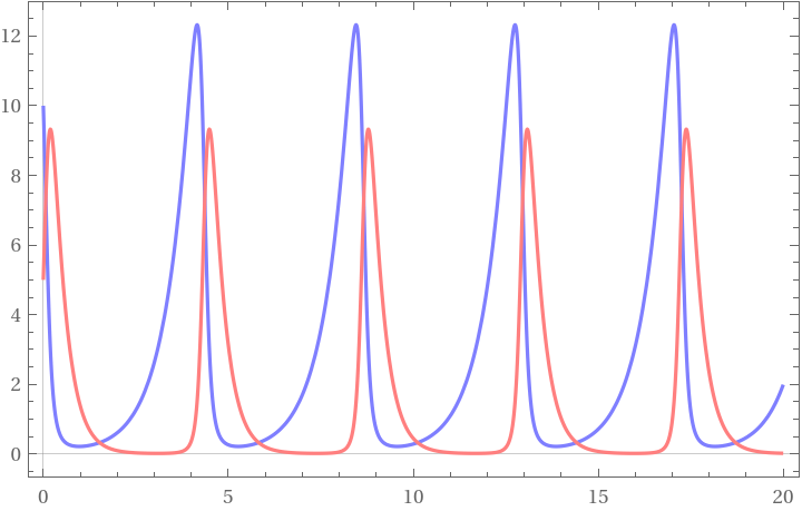
In general, the Lotka-Volterra model refers to the classic two-species construction by Lotka and Volterra, in which the respective instantaneous rates of population change of a predator and prey species are tied to the other species’ population size. In the two species case, the Lotka-Volterra model usually results in periodic population “boom and bust” cycles in which the predator population closely follows but lags behind the prey’s (Bacaër 2011).
Lotka proposed the classic formulation of the model in 1910 as a model of autocatalytic chemical reactions (Lotka 1910). In 1920, he applied the model to a two species food chain involving an idealised plant species and grazing predator (Lotka 1920). In 1925, Volterra independently began studying predator-prey interactions and published a short discussion of the subject in 1926 (Bacaër 2011). While Volterra’s work on the subject focused strictly on modelling predator-prey interactions in fisheries (Volterra 1927), Lotka took a broader interest in exploring competitive interactions and studying the “energetics of evolution” (Lotka 1922). He argued that natural selection could be understood as a physical principle as general as the laws of thermodynamics (Kingsland 2015).
Lotka’s work is noteworthy beyond its contributions to the fields of theoretical population ecology, physical chemistry, and dynamical systems (non-exhaustive) for its interdisciplinarity. He envisioned and worked to create a new biological discipline, “physical biology”, which would apply physical principles and techniques to the study of biological systems composed of processes involving the exchange of matter or energy between system components (Kingsland, 2015). Lotka collected and published these ideas in Elements of Physical Biology (1925).
Lotka-Volterra models serve as critical conceptual tools for ecologists, lending remarkable insights into real-world ecological system dynamics. Its simplicity makes it an excellent choice to demonstrate key ideas about predator-prey interactions, including the influential concept of the prey-predator cycle, whereby prey abundance increases followed by a delayed increase in predators. Its principles have been refined and extended by many subsequent researchers and continue to hold relevance. The primary contribution of the Lotka-Volterra model to the field of ecology is the theoretical underpinning it provides for understanding interspecies interactions, (mainly predation and competition). This fundamental understanding has guided the development of more complex models for describing the dynamics of entire ecosystems.
How does it work?
How does it work?
Consider two species, one which preys on the other (for example, the Canada lynx and snowshoe hare). Let x(t) be the population density of the prey, and y(t) be the population density of the predators at time t. To capture how the populations of each species will vary over time, we need two kinds of information:
1
.The growth rates of the species population in the absence of the other species.
2
.The effect of the presence of the other species on each species’ growth.
In the classic formulation by Alfred J. Lotka, (1920), these parameters are a, b, c, and d, where:
◼
a is the intrinsic growth rate of the prey species
◼
b is the effect of the predators on the prey species growth rate; the rate at which predators kill prey
◼
c is the death rate of the predator species when there are no prey
◼
d is the effect of the prey on the predator species growth rate; the rate at which the predator population grows from consuming prey
Using these parameters, we can write the coupled system of ordinary differential equations:
dx
dt
dy
dt
We assume that each of these parameters is positive. The terms -b x y and d x y indicate that the larger prey and predator species are, the higher the mass/population/energy transfer from prey to predators will be.
Implementation: In the Wolfram Language
Implementation: In the Wolfram Language
Setting up a Lotka-Volterra model in the Wolfram Language is very straightforward using , WL’s numerical differential equations solver.
1
.Since we know the model takes two initial conditions (species population sizes) and four parameters (a, b, c, d), we can write a helper function that takes in this information and returns the appropriate coupled equations:
Set up the ODEs and initial conditions describing a two-species Lotka-Volterra model:
In[]:=
ClearAll[lotkaVolterra]lotkaVolterra[{xInit_,yInit_},{a_,b_,c_,d_}]:={(*prey population*)x'[t]==a*x[t]-b*x[t]*y[t],(*predator population*)y'[t]==-c*y[t]+d*x[t]*y[t],(*Initial conditions*)x[0]==xInit,y[0]==yInit}lotkaVolterra[]:=lotkaVolterra[{xInit,yInit},{a,b,c,d}]
Example:
Column[lotkaVolterra[{10,5},{1.5,1,3,1}]]
Out[]=
′ x |
′ y |
x[0]10 |
y[0]5 |
2
.Now, we can simply call our helper function inside NDSolve, specifying our initial conditions and parameters. Additionally, we supply a list of variables to solve for, and another containing the name and range of the independent variable, t.
sol=NDSolve[lotkaVolterra[{10,5},{1.5,1,3,1}],{x,y},{t,0,20}]
Out[]=
xInterpolatingFunction,yInterpolatingFunction


3
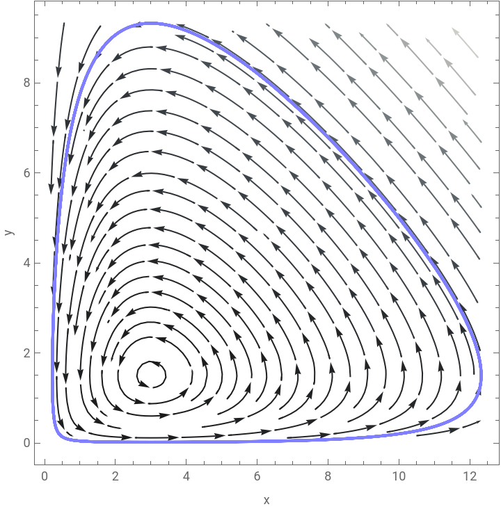
.Finally, we can plot these results in the time domain and state space:
Time domain plot:
Out[]=


State space portrait:
Out[]=

Bonus: Explore it yourself using Manipulate
Bonus: Explore it yourself using Manipulate
Relationships and Food Webs
Relationships and Food Webs
Predation Relationships and Food Webs
Predation Relationships and Food Webs
Suppose we would like to extend our model to three or more species. For a given n-species system, will need too keep track of the relationships between species, and their effects on one another. We will discuss two ways of storing this information: one to facilitate our conceptual understanding of model configurations, and the other to facilitate the process of building the model system of ODEs. We will discuss the first of these ways here.
Notice that as the number of species n in our model grows, so does the number of possible relationships between species (at a rate of , or if we assume the absence of cannibalism in the community). The number of possible combinations of relationships also grows without bounds (at a rate of , or without cannibalism). A set of predation relationships between species is known as a food web.
n
2
n-1
2
2
n
2
2
(n-1)
2
In a food web, predation relationships are usually represented as arrows from prey to predator species, representing transfer of energy up the web’s component food chains.
A simple 3-species food web:
Out[]=
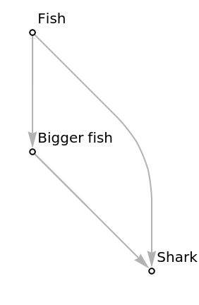
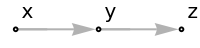
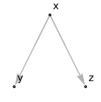
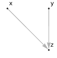
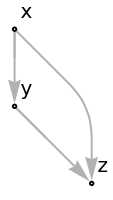
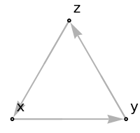
Since food webs are graphs, we can express them directly in the Wolfram Language using Graph objects (see documentation: ). Not all food web configurations will be ecologically meaningful, and some will be analogous to one-another, but expressing them like this helps to get a strong qualitative impression of the relationships they depict (Are we modelling a really simple web, or is it very complicated? How tangled is it? How loopy? How close together are the species? Do they form clusters? And so on). We can also answer questions about the food web parameter spaces. For instance: what structurally distinct categories of 3-species food web are there?
Categories of three species food webs (Hsu, Ruan, and Yang 2015):
Aside: What species relationships are possible in an n-species system?
Aside: What species relationships are possible in an n-species system?
We can write a function to generate the possible predation configurations for a species in an n-species food web:
Predation configurations for a species in an n-species food web:
We can sample possible food web configurations randomly, but this will rarely yield realistic food webs for most contexts. Instead, we might restrict configurations to a subset of forms that fit our criteria, or we might simply look to real world systems for examples.
Random valid 3-species food webs (with cannibalism):
Random valid 3-species food webs (without cannibalism):
Species to Species Effects Representation: The Community Matrix
Species to Species Effects Representation: The Community Matrix
Whereas graphs are great at helping us intuit the nature of interactions in a community, we typically express interactions in n-species Lotka-Volterra models using a matrix of interaction coefficients called an interaction matrix. A perk of this strategy is that it allows us to write the generalised Lotka-Volterra model in a condensed form using linear algebra. We will discuss this condensed form shortly. When the matrix stores the effects of species on other species growth rates, we call this matrix a community matrix.
An example Community/Interaction matrix:
In the following sections, I have implemented some simple tools to translate between community matrices and food webs.
Three+ species Lotka-Volterra
Three+ species Lotka-Volterra
Generalised Lotka-Volterra: How Does it Work?
Generalised Lotka-Volterra: How Does it Work?
We can model competition and predation systems with more than two species using the generalised form of the Lotka-Volterra model, which we write:
where
We will define the intrinsic growth rates slightly differently from our approach for the two-species model, as we assume that each species has a positive intrinsic growth rate. We account for the negative effect of a species’ intraspecific competition in the absence of food (on its intrinsic growth rates) in the diagonal of the community matrix.
Three Species Lotka-Volterra in the Wolfram Language
Three Species Lotka-Volterra in the Wolfram Language
Numerical Approximation of Generalised Lotka-Volterra Dynamics
Numerical Approximation of Generalised Lotka-Volterra Dynamics
We can compose the GeneralizedLotkaVolterraODEs function defined in the previous subsection with NDSolve to numerically approximate the trajectories of arbitrary three-species Lotka-Volterra models. The process is the same as for the two-species model.
We can use GeneralizedLotkaVolterraODEs to generate the system of ODEs for the given initial parameters:
◼
vars - a list of variable names (optional),
◼
init - a list of initial population sizes
◼
r - a list of species intrinsic growth rates
◼
interactionMatrix - a matrix describing community interactions (in our examples, a community matrix)
Generate a system of ODEs for a Generalised Lotka-Volterra model from provided parameters:
Using CommunityMatrixGraph, we can construct a weighted graph from the community matrix to get an idea of the relationships that define the system at a glance.
Visualise the community interactions described by the community matrix:
And NDSolve to numerically approximate the population trajectories of the model.
Numerical solutions to the model ODEs:
We can then plot the solutions in the time domain and state space:
Time domain plot:
State space portrait (now in 3D!):
Closing Notes: Four species and more
Closing Notes: Four species and more
The generalised model we have discussed in this short text extends beyond three species systems. In fact, the tools we have developed will allow us to model any finite n-species closed-food web, that is, any system that we can express using a finite number of species initial population sizes, intrinsic growth rates, and interactions. It should be noted that just because we can specify a model does not always mean we can accurately solve for its behaviour: we are restricted by the limits of numerical approximation and our available computational power)
Still, we can easily model four species webs. Let’s make prepare two four species models. We’ll define some weighted webs describing the various interaction effects of our system:
We can construct the community matrix describing either of these using the CommunityMatrix function. For example, take the first row of interaction webs from the above dataset:
We model following the model construction steps discussed in the previous section.
Explore the models in the time domain:
Note: What happened to the state-space plot? Well, we’ve run out of spatial dimensions to express the behaviour of the system, and in the interest of keeping this post short, we’ll leave things there for now.
Consider what we have achieved in this short text. If you have read this far, I hope to have inspired you think of how you might answer your own ecological questions in the Wolfram Language. If your questions expand on the subject of this post, I hope the tools I have developed within will help jumpstart your exploration! And please, don’t hesitate to reach out to me with any questions you may have about this work.
CITE THIS NOTEBOOK
CITE THIS NOTEBOOK
Lotka-Volterra Models in the Wolfram Language
by Phileas Dazeley-Gaist
Wolfram Community, STAFF PICKS, October 6, 2023
https://community.wolfram.com/groups/-/m/t/3028599
by Phileas Dazeley-Gaist
Wolfram Community, STAFF PICKS, October 6, 2023
https://community.wolfram.com/groups/-/m/t/3028599