This notebook explores the quantum Fisher information (QFI) for photonic states in quantum optics, using the Fubini–Study metric to quantify parameter sensitivity. Various one- and two-mode states are analyzed to illustrate their metrological potential and possible enhancements beyond the standard quantum limit. This analysis can be extended to do computational explorations of other photonic states in quantum metrology.
Install the Wolfram Quantum Framework:
In[]:=
PacletInstall["https://www.wolfr.am/DevWQCF",ForceVersionInstall->True]
Out[]=
PacletObject

Load the functionalities:
In[]:=
<<Wolfram`QuantumFramework`<<Wolfram`QuantumFramework`SecondQuantization`<<Wolfram`QuantumFramework`QuantumOptimization`
Quantum Fisher Information
Quantum Fisher Information
A classical statistical definition of Fisher information to estimate some parameter θ that has a probability distribution is:
p(x|θ)

The Quantum Fisher Information (QFI) quantifies the maximum amount of information about an unknown parameter θ that can be extracted from a quantum measurement on a state ρ(θ). It sets a lower bound on the variance of any unbiased estimator of via the quantum Cramér-Rao Bound:

In quantum optics, a parameter that is typically chosen for estimation is the phase. Depending on the state used, there are limits that dictate bounds on how accurately this parameter can be estimated.
An interesting mathematical property of the Fisher information is its relation to the Fubini-Study metric tensor. If a quantum state is parametrized by a parameter θ, the following relation holds
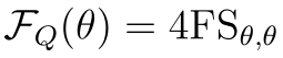
where is the diagonal element of the tensor associated to the parameter θ, if the state only has one parameter the tensor is a scalar
FS
θ,θ
Single mode states
Single mode states
Two state Fock superposition
Two state Fock superposition
Lets analyze the state

Pick random values of and :
n
m
In[]:=
{n,m}=RandomSample[Range[1,$FockSize-1],2];
Build the state :
In[]:=
ψ=QuantumStateCos[α]FockState[n]+Sin[α]FockState[m],"Parameters"->{α,δ}
δ
Out[]=
cos(α)|5〉+sin(α)|10〉
δ
The state has two parameters , so FubiniStudyMetricTensor returns a 2x2 matrix. We can get the Fisher information from the diagonal element of the tensor associated to the θ parameter (check documentation ):
Extracting the quantum Fisher information for both parameters:
In[]:=
QFI=4Simplify[Normal@Diagonal[FubiniStudyMetricTensor[ψ]["Matrix"]],Element[{α,δ},Reals]];
For α parameter the Quantum Fisher information is constant and its value is related to the maximal of Fisher information for two dimensional subspace (similar to a qubit in Bloch sphere). For the relative phase parameter δ the Fisher information has dependance on α, note that for the superposition is lost and global phases cannot be measured
α=0orα=π/2
Define a qubit state:
In[]:=
qubitState=QuantumStateCos[α],Sin[α],"Parameters"->{α,δ};
δ
Quantum Fisher information for the two level state:
In[]:=
qubitQFI=4Simplify[Normal@Diagonal[FubiniStudyMetricTensor[qubitState]["Matrix"]],Element[{α,δ},Reals]];
Check the Fisher information related to both parameters is the same:
In[]:=
QFI-qubitQFI
Out[]=
{0,0}
Plot the Crámer-Rao bound, also note the result does not depend on the and m chosen:
n
In[]:=
Plot3DEvaluate,{α,0,π/2},{δ,0,2π},
1
QFI
Out[]=


Coherent state
Coherent state
In[]:=
SetFockSpaceSize[30];
Phase shifted coherent state:
In[]:=
ψ=QuantumStateCoherentState[][α],"Parameters"->{α,θ};
θ
Norm of the state:
In[]:=
norm=CoherentState[][α]["Norm"];
Get the Quantum Fisher information:
In[]:=
QFI=Simplify[4FubiniStudyMetricTensor[ψ/norm]["Matrix"][[2,2]],θ∈Reals];
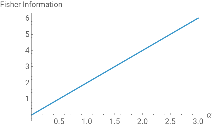
The Fisher information has quadratic dependence on |α|, or linear with |α(SQL) :
2
|
In[]:=
Plot
QFI
,{α,0,3.},LabelStyle->13,AxesLabel->{"α","Fisher Information"}Out[]=
Squeezed vacuum state
Squeezed vacuum state
Squeezed vacuum with real squeeze parameter, phase shifted:
In[]:=
ψ=QuantumState[PhaseShiftOperator[θ]@SqueezeOperator[r][],"Parameters"->{r,θ}];
Quantum Fisher information:
In[]:=
QFI=4(FubiniStudyMetricTensor[ψ]["Matrix"][[2,2]]/.Conjugate[θ]->θ);
The resulting Quantum Fisher information has functional form , is expected to be a function of Sinh since = for a squeezed vacuum state:
2
2
Sinh[2r]
—
n
2
Sinh[r]
In[]:=
data=Table[{rs,Re[QFI/.r->rs]},{rs,0.001,0.6,0.001}];NonlinearModelFit[data,A,{A,B,F},r]["BestFitParameters"]
F
(Sinh[Br])
Out[]=
{A2.00002,B1.99999,F2.}
Plot the Fisher information and CR bound:
In[]:=
PlotQFI,,{r,0,1},
1
QFI
Out[]=
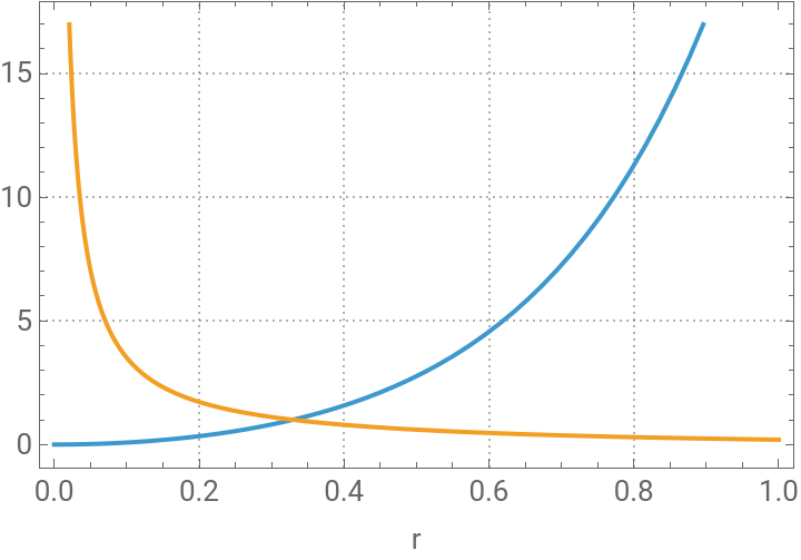


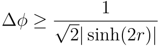
Hence for large there is notable phase sensitivity, that is why squeezed states are used in many important experiments (LIGO for example). Makes sense because for an squeezed vacuum the mean number of photons is , and Sinh[2r] behaves asymptotically as so this is close to the Heisenberg limit.
r
2
Sinh[r]
2
Sinh[r]
1
N
Two mode states
Two mode states
NOON state
NOON state
In[]:=
SetFockSpaceSize[20];
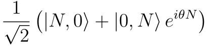
A NOON state is defined as the superposition :
In[]:=
NOONstate[N_,size_:$FockSize]:=QuantumStateFockState[{N,0},size]+FockState[{0,N},size],"Parameters"->θ
1
2
Nθ
NOON state with N = 2:
In[]:=
ψ=NOONstate[2]
Compute Quantum Fisher Information from the FubiniStudyMetricTensor, for different NOON states:
Consider N = 10:
Obviously these states are orthogonal:
The associated measurement probabilities are:
Entangled coherent states
Entangled coherent states
Normalization constant for the whole state:
Normalized state:
Quantum Fisher information, using the Fubini Study Metric Tensor:
Analytical result of the Crámer-Rao bound:
There is a threshold value of |α| such the numerical error increases monotonically due to truncation effects:
Twin Fock State
Twin Fock State
Annihilation operators for two modes:
Define a twin Fock state for N = 4:
A twin Fock state is unaffected by this operation(no phase sensitivity):
Compute the QFI for different twin Fock states after beam-splitter evolution:
Resulting functional form, similar to NOON state but it has a reduced prefactor, here N is the total number of photons:
Spin Husimi Function for state |4,4〉
Mapping the state after the beam-splitter operation:
Now for this state the spin Husimi function has ϕ dependence:
Fock-coherent state
Fock-coherent state
A Fock-coherent state is defined as |N〉 ⊗ |α〉, where N is any Fock state number:
Two mode operators:
Coherent state norm:
Compute the Fisher information:
CITE THIS NOTEBOOK
CITE THIS NOTEBOOK
Computing the quantum Fisher information via the Fubini–Study metric for photonic states
by Bruno Tenorio
Wolfram Community, STAFF PICKS, October 16, 2025
https://community.wolfram.com/groups/-/m/t/3561108
by Bruno Tenorio
Wolfram Community, STAFF PICKS, October 16, 2025
https://community.wolfram.com/groups/-/m/t/3561108