Alma Fluida Navier Stokes equations with periodic boundary conditions
by Pietro G. Fré & Mario Trigiante ⋆
University of Torino, Department of Physics, Via P. Giuria, 1, I-10125 Torino, Italy. email: pietro.fre@unito.it
⋆ Politecnico di Torino, DISAT, C.so Duca degli Abruzzi,24, I-10129, Torino, Italy. email: mario.trigiante@polito.it
by Pietro G. Fré
University of Torino, Department of Physics, Via P. Giuria, 1, I-10125 Torino, Italy. email: pietro.fre@unito.it
⋆ Politecnico di Torino, DISAT, C.so Duca degli Abruzzi,24, I-10129, Torino, Italy. email: mario.trigiante@polito.it
The calculation codes here presented are organized in a coherent system of WOLFRAM MATHEMATICA Notebooks and are devoted to Navier Stokes Equations with Periodic Boundary Conditions. The Alma Fluida NSP System is an instrument for the mathematical study of NS equations within the previously unknown Group Theoretical Framework provided by the notion of the Universal Classifying Group, introduced by P.Fré and A.S. Sorin in 2015 and further developed, extended, completed and systematized by the two present authors in a new publication on the ArXive entitled “Chaos from Symmetry: Navier Stokes equations, Beltrami fields and the Universal Classifying Crystallographic Group”:
https://arxiv.org/abs/2204.01037
https://arxiv.org/abs/2204.01037
Highlights of the Theory presented in Chaos from Symmetry
Highlights of the Theory presented in Chaos from Symmetry
From the abstract
From the abstract
The general set up for the classification and construction of Arnold-Beltrami Flows on three dimensional torii is revised, reorganized and completed.The focal idea of a Universal Classifying Group UCG for crystallographic lattices is duly improved and extended. We constructed the missing UCG for the hexagonal lattice and mastering the cubic and hexagonal instances of this group, we can cover all cases.
TheUCGforthecubiclatticeis=solvablegroupwith1536elements,37conjugacyclassesand37irreps;∼(×××)
G
1536
G
1536
S
4
×
semidirect
4
4
4
4
TheUCGforthehexagonallatticeis=solvablegroupwith72elements,24conjugacyclassesand24irreps;∼(×)
U
72
U
72
2
×
semidirect
6
6
The upgrading of Beltrami Flows to a special type of periodic solutions of the Navier Stokes equations is presented and the relation between the classification of Beltrami Flows with the classification of contact structures is enlightened. The recent developments in contact and symplectic geometry that allow the consideration of singular contact structures and Beltrami fields in the framework of b-manifolds with distinguished critical surfaces is reviewed and it is shown that the choice of the allowed critical surface for the b-deformation of a Beltrami field seems to be strongly related with its group-theoretical structure. The Landscape conception of spherical layers in the dual momentum lattice as main token for the construction of Beltrami fields is clarified and established on general grounds.
From the conclusions
From the conclusions
The Beltrami operator is a chiral one. There are solutions with ±λ where λ is an admissible eigenvalue. Hence the conventional Fourier expansion of any periodic field can be subdivided in two parts the Beltrami plus and the Beltrami minus part (or anti-Beltrami). It was advocated in the following old paper
P. Constantin and A. Majda, “The beltrami spectrum for incompressible fluids”, Communications in Mathematical Physics, vol. 115, p. 864 - 896, 1988.
Beltrami fields weakly interact among themselves and one can define and index of Beltramicity per frequency that is approximately conserved in time. This viewpoint can be very fertile in dealing with the group theoretical construction of Beltrami fields. In the landscape approach we are free to sum exact solutions only in a definite spherical layer. If we mix different layers we obtain objects that are not exact solutions. Yet the weak interaction viewpoint suggests that such sums can approximate exact solutions in a nice and controllable way. This is a very much promising direction of research if the summation on layers is organized in irreps of the UCG group or suitable subgroups thereof.
From figures obtained with the Alma Fluids NSP system
From figures obtained with the Alma Fluids NSP system
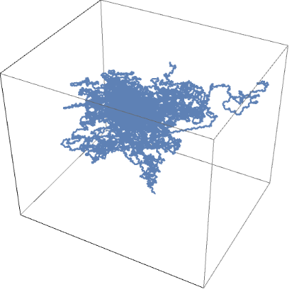
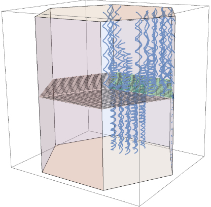
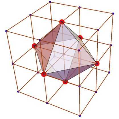
In the following slot we show three illustrative figures. The first is a single chaotic trajectory in the fundamental cell of the cubic torus, produced by a Beltrami velocity field. The second is a set of spiraling trajectories produced by a Beltrami velocity field in the hexagonal lattice. The third is a length 6 orbit of the octahedral point group in the cubic momentum lattice.
Structure and installation of the Alma Fluida NSP system
Structure and installation of the Alma Fluida NSP system
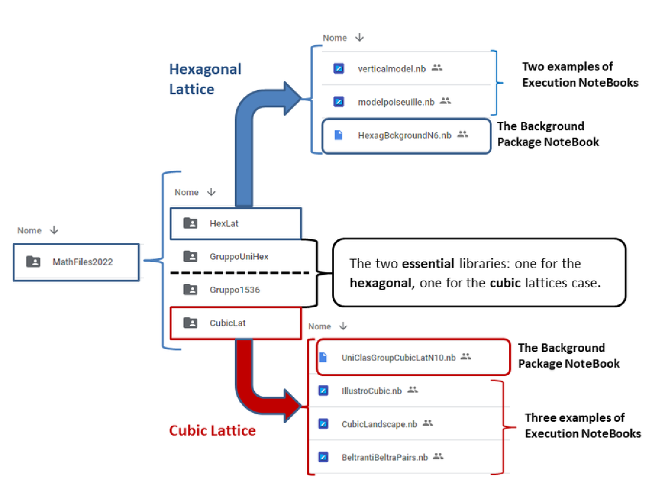
The calculation system Alma Fluida NSP is composed of two Bakground NoteBooks, respectively dealing with the case of the Cubic Lattice and of the Hexagonal Lattice:
1
.UniClasGroupCubicLatN10.nb
2
.HexagBckgroundN6.nb
that contain all the routines and subroutines of the system plus a theoretical summary and a very much extended User Guide for each one of the two cases.
In addition the system comprises two libraries of data, one for the cubic case, one for the hexagonal one that contain essential information in order for either one of the two systems to work, as the list of elements organized in conjugacy classes of the two universal class groups, the list of all their irreps and the correspondence rules to obtain the matrix representation of each group element in each irrep, the character tables, the list of relevant subgroups and the directives to create branching rules.
In addition the system comprises two libraries of data, one for the cubic case, one for the hexagonal one that contain essential information in order for either one of the two systems to work, as the list of elements organized in conjugacy classes of the two universal class groups, the list of all their irreps and the correspondence rules to obtain the matrix representation of each group element in each irrep, the character tables, the list of relevant subgroups and the directives to create branching rules.
In order to work with either one of the two Codes (Cubic or Hexagonal) the User should have downloaded on his/her computer the folder MathFiles2022 whose structure is displayed below
The full folder is available and you can get it freely from the Personal Google Drive Repository of Prof. Pietro Fré on the University of Torino Server, using the link:
https://drive.google.com/drive/folders/1hDz4dRmcTOYBrK7jKpUr2xmbc9GO4zUh?usp=sharing
https://drive.google.com/drive/folders/1hDz4dRmcTOYBrK7jKpUr2xmbc9GO4zUh?usp=sharing
Installation instructions
Installation instructions
After you have obtained the entire MathFiles2022 folder you save it as it stands, without altering anything of its internal structure, in your favorite working directory
XXXXXXXXXXX
XXXXXXXXXXX
In each of the two background NoteBooks you find a preliminary section like the following one that applies to the cubic case
Directory
Directory
Before evaluation of this Notebook on other computers you need to install on your computer the folder MathFiles2022 .
You can download the folder Mathfiles2022 from the following link
download Mathefiles2022 from google drive
You can download the folder Mathfiles2022 from the following link
download Mathefiles2022 from google drive
Setting the Directory and the Library
Setting the Directory and the Library
After installation of the folder MathFiles2021 and before the evaluation of this Notebook on other computers you need to write here the address of your working directory where the MathFiles2021 directory has been deployed. Follow the example.
Writing the user's addresses
Writing the user's addresses
In[]:=
direchome="C:\Users\718290\Documents\CurrentWork\AlmaFluidaNSP\MathFiles2022\Gruppo1536";
In[]:=
direcyours="XXXXXXXXXXXXXXX\MathFiles2022\Gruppo1536";
Choosing the working directory
Choosing the working directory
Here instead of direc=direchome, which is the working directory of the author you will write direc=direcyours or whatever different name you want to give to your working directory. Note that you can list at the beginning several different direc addresses (with different names) if you work on different computers and each time you just change the statement direc=direcwhatever and you become operative on the different computer.
direc=direcyours
Out[]=
C:\Users\718290\Documents\CurrentWork\AlmaFluidaNSP\MathFiles2022\Gruppo1536
After these operations have been completed you can Evaluate the Notebook. All routines and commands will be operating. You will work in other Notebooks and the first instruction will always be initializer or initializermute. This will upload all the necessary information and create all the needed items for the other routines and commands to function
Working with the system
Working with the system
From your reading of the first section in each of the two background NoteBook you will learn all what you can do with each one. The important warning is that before Evaluating either one of the two background NoteBooks you should Quit Kernel. The two subsystems, for the Cubic Lattice and for the Hexagonal Lattice are self-consistent but interfere destructively with each other.
You can get a flavor of the possibilities by looking at one of the examples contained in the directory CubicLat, for instance the Execution NoteBook Illustrocubic.nb
Examples
We assume that you have evaluated the background NoteBook HexagBckgroundN6.nb with your working directory correctly assigned:
direcyours=”XXXXXXXXXXXXXXXXXXXXXXXXXXX\MathFiles2022\GruppoUniHex”;
and the instruction:
direc=direcyours
direcyours=”XXXXXXXXXXXXXXXXXXXXXXXXXXX\MathFiles2022\GruppoUniHex”;
and the instruction:
direc=direcyours
Classical solution of NS equation
Classical solution of NS equation
We recall the classical solution of NS equation named after Poiseuille in a cylindrical tube.
The velocity field is of the form
U=={0,0,f(x,y)}
w
3
f(x,y)
2
The pressure field is of the form
p=p(z)=az+b
It easily follows that
U·∇U≡=0
U
[U]
dΩ
Hence the equation reduces to
νf(x,y)-=0
Δ
2
∂p(z)
∂z
where
Δ
2
2
∂
∂
2
x
2
∂
∂
2
y
is the two - dimensional Laplacian
Setting :
f(x,y)=--
2
R
2
x
2
y
2
We find :
νf(x,y)+f(x,y)=-2
2
∂
∂x∂x
2
∂
∂y∂y
2
ν=aHence the complete solution of the steady Navier Stokes equations named after Poiseuille is the following
U=0,0,--;p=-2
2
R
2
x
2
y
2
2
νz+p
0
WhereRistheradiusofthecirculartubeandistheinitialpressure
p
0
Hexagonal Poiseuille
Hexagonal Poiseuille
We show how to adapt that solution to a tube with a hexagonal section in the fundamental cell of the hexagonal lattice
The basis vector of the lattice are recalled here
In[]:=
ww
Out[]=
,,0,0,0,
2
,0,0,-1
2
3
2
2
Running the routine hexagpoiseul
Running the routine hexagpoiseul
Running initiomute
Running initiomute
We initialize the background programme for Beltrami solutions
Analysis of a singlet solution
Analysis of a singlet solution
Instead of calculating a Beltrami vector field that happens to be in a singlet of the Universal Classifying Group, operation that would take too much space in this exemplification post, we import it from separate calculations
Plot of this vector field
Plot of this vector field
Calculation and visualization of streamlines with the graphical routine mainvisualizehexag
Calculation and visualization of streamlines with the graphical routine mainvisualizehexag
Running the principal routine
Inserting the specific vector field
A neutral substitution rule
Running the routine preparosolhexag