ABSTRACT (original article): We present a comprehensive study surface plasmon polariton (SPP) propagation on planar metallic waveguides under a dressing field. We perform a set of analytical calculations of the periodic time-dependent Schrödinger equation to study the interaction of an intense electromagnetic field with a metallic system. We model the strong light coupling to the metallic system using a nonperturbative procedure. In this paper, we show that, by introducing Floquet theory into the dressed metal, the behavior of the Floquet states are similar to the phase-modulated signals in the communication system. This will reveal a new perspective on the underlying science in an intricate dressed quantum system. Furthermore, we examine the impurity scattering effects on charge transport in disordered plasmonic metals using the generalized Floquet-Fermi golden rule, and provide a novel approach to diminish the losses in plasmonic materials using the dressing field. To gauge the effectiveness of our results, we introduce a figure of merit (FOM) to compare the performance of plasmonic metals, subjective to a dressing field. The calculated dressed SPP characteristics suggest that high-efficiency SPP propagation can be achieved in practice. Our findings open up new directions for state-of-the-art nanoplasmonic devices. CITATION (original article): Herath, K. & Premaratne, M. Floquet engineering of dressed surface plasmon polariton modes in plasmonic waveguides. PHYSICAL REVIEW B 106, 235422 (2022). https://doi.org/10.1103/PhysRevB.106.235422
Import external libraries and define global parameters
Import external libraries and define global parameters
Import external libraries: MaTex to include latex wording into the diagrams and CustomTicks to customize the ticks in plots.
In[]:=
ClearAll["Global`*"]Needs["MaTeX`"]Needs["CustomTicks`"]imageScale=72/2.54;
Define parameters
Define parameters
Define the all parameters we used in this calculation.
Physical constants
Physical constants
These are physical constant that will not be changed through out the calculation.
e=Quantity[(1.602176)*10^(-19),"Coulombs"];(*electron'scharge*)hbar=Quantity[(1.054571)*10^(-34),("Kilograms"*"Meters"^2)/"Seconds"];(*Plank'sconstant*)m=Quantity[(9.109383)*10^(-31),"Kilograms"];(*electron'smass*)c=Quantity[(2.997924)*10^(8),"Meters"/"Seconds"];(*speedoflightinvacuum*)ϵ0=Quantity[(8.854187)*10^(-12),("Coulombs"^2*"Seconds"^2)/("Kilograms"*"Meters"^(3))];(*vacuumpermittivity*)eV=Quantity[(1.602176)*10^(-19),("Kilograms"*"Meters"^2)/("Seconds"^(2))](*electronVolts*)
System parameters - dressing field
System parameters - dressing field
These are parameters that are related to the dressing field.
FieldInt0=Quantity[(1)*10^(3),"Kilograms"/"Seconds"^(3)];(*Referencedressingelectricfield'sintensity=0.1*)ω=Quantity[(1.35)*10^(12),"Seconds"^(-1)](*Dressingfield'sfrequency=1.35×*)
-2
Wcm
12
10
-1
rads
System parameters - SPP wave
System parameters - SPP wave
Here we define the parameters that are related to the SPP initiating field.
λspp=Quantity[(633)*10^(-9),"Meters"];(*SPPwavewavelength*)ωspp=(2*π*c)/λspp;(*SPPwavefrequency*)
Numerical Analysis - Silver (Ag)
Numerical Analysis - Silver (Ag)
We calculate basic numerical values for different optical properties of silver.
Experimental material parameters
Experimental material parameters
Related empirical parameters of silver.
me=1*m;(*Effectiveelectron'smassforSilver=1m*)EFermi=5.5*eV;(*FermienergyforSilver=5.5eV*)kFermi=Sqrt[2*EFermi*me/(hbar^2)];(*FermiwavenumberforSilver*)
Additional parameters
Additional parameters
Here we define system parameters that related the system.
In[]:=
q=1;(*Dressingfield'sintensitymultiplication*)FieldInt=q*FieldInt0;Eamp=Sqrt[(2*FieldInt)/(c*ϵ0)];(*Dressingelectricfield'samplitude*)λ=e/(me*ω^2);(*Pre-definedparameter*)ξ=λ*Eamp*kFermi(*Pre-definedparameter*)
Out[]=
1.00648
Frequency spectrum analysis of Floquet states
Frequency spectrum analysis of Floquet states
Define the summation of zeroth order Bessel function.
In[]:=
J[μ_,λ_,n_]:=Sum[BesselJ[(n-2*l),μ]*BesselJ[l,λ],{l,-10,10}];
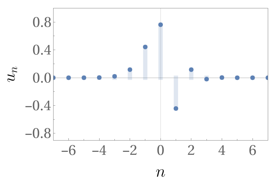
Frequency spectrum: I =I0
Frequency spectrum: I =I0
Frequency spectrum calculation the applied field’s intensity is equals to the reference intensity:
Er=Sqrt[(2*FieldInt0*1)/(c*ϵ0)];(*Dressingelectricfield'samplitude*)γ=-(e*Er)/(hbar*ω);μ1=(hbar*γ*kFermi)/(me*ω);(*GBFfirstargument*)λ1=(hbar*γ^2)/(8*me*ω);(*GBFsecondargument*)
In[]:=
S1=DiscretePlot[J[μ1,λ1,n],{n,-7,7},AxesFalse,GridLines{{{0,Gray}},{{0,Black}}},PlotStyleThickness[0.02],PlotMarkers{Automatic,9},PlotRange{{-7,7},{-0.9,1}},Frame{{True,True},{True,True}},FrameTicksStyle{{FontSize24,None},{FontSize24,None}},FrameTicks{{LinTicks[{-0.8,-0.4,0,0.4,0.8},Range[-0.8,1.0,0.2]],None},{LinTicks[{-6,-4,,-2,0,2,4,6},Range[-7,7,1]],None}},FrameLabel{{MaTeX["u_{n}",FontSize28],None},{MaTeX["n",FontSize28],None}},LabelStyle{{{FontFamily"Times New Roman"},None},{FontFamily"Times New Roman",None}},ImageSize12*imageScale]
Out[]=
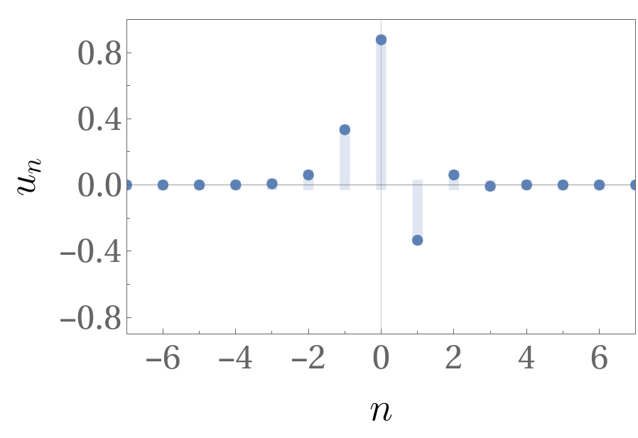
Frequency spectrum: I =0.5*I0
Frequency spectrum: I =0.5*I0
Frequency spectrum calculation the applied field’s intensity is equals to the half of the reference intensity :
Er=Sqrt[(2*FieldInt0*0.5)/(c*ϵ0)];(*Dressingelectricfield'samplitude*)γ=-(e*Er)/(hbar*ω);μ1=(hbar*γ*kFermi)/(me*ω);(*GBFfirstargument*)λ1=(hbar*γ^2)/(8*me*ω);(*GBFsecondargument*)
In[]:=
S2=DiscretePlot[J[μ1,λ1,n],{n,-7,7},AxesFalse,GridLines{{{0,Gray}},{{0,Black}}},PlotStyleThickness[0.02],PlotMarkers{Automatic,9},PlotRange{{-7,7},{-0.9,1}},Frame{{True,True},{True,True}},FrameTicksStyle{{FontSize24,None},{FontSize24,None}},FrameTicks{{LinTicks[{-0.8,-0.4,0,0.4,0.8},Range[-0.8,1.0,0.2]],None},{LinTicks[{-6,-4,,-2,0,2,4,6},Range[-7,7,1]],None}},FrameLabel{{MaTeX["u_{n}",FontSize28],None},{MaTeX["n",FontSize28],None}},LabelStyle{{{FontFamily"Times New Roman"},None},{FontFamily"Times New Roman",None}},ImageSize12*imageScale]
Out[]=
Frequency spectrum : I = 5*I0
Frequency spectrum : I = 5*I0
Frequency spectrum calculation for the applied field’s intensity is equals to the five times the reference intensity :
Frequency spectrum: I =10*I0
Frequency spectrum: I =10*I0
Frequency spectrum calculation for the applied field’s intensity is equals to the ten times the reference intensity :
Inverse scattering time matrix central element analysis (n=0)
Inverse scattering time matrix central element analysis (n=0)
Here, we calculate the elements of the inverse scattering matrix under different intensities(0.5*I0, I0, 2*I0, and 4*I0). This calculation consider the contribution of the n=0 element:
Inverse scattering time matrix central element analysis (n = 1)
Inverse scattering time matrix central element analysis (n = 1)
Here, we calculate the elements of the inverse scattering matrix under different intensities(0.5*I0, I0, 2*I0, and 4*I0). This calculation consider the contribution of the n=1 element:
Inverse scattering time matrix central element analysis (n = 2)
Inverse scattering time matrix central element analysis (n = 2)
Here, we calculate the elements of the inverse scattering matrix under different intensities(0.5*I0, I0, 2*I0, and 4*I0). This calculation consider the contribution of the n=2 element:
Inverse scattering time matrix central element analysis (n = 3)
Inverse scattering time matrix central element analysis (n = 3)
Here, we calculate the elements of the inverse scattering matrix under different intensities (0.5*I0, I0, 2*I0, and 4*I0) . This calculation consider the contribution of the n = 3 element :
Inverse scattering time matrix central element analysis (n = 4)
Inverse scattering time matrix central element analysis (n = 4)
Here, we calculate the elements of the inverse scattering matrix under different intensities (0.5*I0, I0, 2*I0, and 4*I0) . This calculation consider the contribution of the n = 4 element :
Now, we calculate the elements of the inverse scattering time matrix under different intensities. Here we consider I=I0:
Now, we calculate the elements of the inverse scattering time matrix under different intensities. Here we consider I=16*I0:
Manipulate the Energy Broadening
Manipulate the Energy Broadening
Define the normalized energy band broadening function and calculate its numerical values for different intensity levels with parameters of silver:
Numerical Analysis - Gold (Au)
Numerical Analysis - Gold (Au)
Experimental material parameters
Experimental material parameters
Related empirical parameters of gold.
Additional parameters
Additional parameters
Here we define system parameters that related the system .
Manipulate the Energy Broadening
Manipulate the Energy Broadening
Define the normalized energy band broadening function and calculate its numerical values for different intensity levels with parameters of gold :
Numerical Analysis - Copper (Cu)
Numerical Analysis - Copper (Cu)
Experimental material parameters
Experimental material parameters
Related empirical parameters of copper.
Additional parameters
Additional parameters
Here we define system parameters that related the system .
Manipulate the Energy Broadening
Manipulate the Energy Broadening
Define the normalized energy band broadening function and calculate its numerical values for different intensity levels with parameters of copper :
Numerical Analysis - Aluminum (Al)
Numerical Analysis - Aluminum (Al)
Experimental material parameters
Experimental material parameters
Related empirical parameters of aluminum.
Additional parameters
Additional parameters
Here we define system parameters that related the system .
Manipulate the Energy Broadening
Manipulate the Energy Broadening
Define the normalized energy band broadening function and calculate its numerical values for different intensity levels with parameters of aluminum :
SPP Manipulation - All metals (Ag, Au, Cu, Al)
SPP Manipulation - All metals (Ag, Au, Cu, Al)
In this part of the analysis, we consider to calculate the optical and related SPP properties of each given plasmonic metal.
Experimental material parameters
Experimental material parameters
First, we define the empirical parameters of each metal and calculate their natural dielectric function values using the Drude mode:
Silver
Silver
Dielectric function natural real part(ϵ ‘)
Dielectric function natural imaginary part(ϵ ‘’)
Gold
Gold
Dielectric function natural real part(ϵ ‘)
Dielectric function natural imaginary part(ϵ ‘’)
Copper
Copper
Dielectric function natural real part(ϵ ‘)
Dielectric function natural imaginary part(ϵ ‘’)
Aluminum
Aluminum
Dielectric function natural real part(ϵ ‘)
Dielectric function natural imaginary part(ϵ ‘’)
Normalized Energy Band Broadening (Figure 05)
Normalized Energy Band Broadening (Figure 05)
Calculated data from the inverse scattering time calculations from above section’s Tables. Here we used them analyze these data separately.
Generate data pairs to draw the plots.
The normalized total energy band broadening vs the normalized dressing field’s intensity plot for silver, gold, copper and aluminum:
Save the graph in PDF format.
Normalized SPP Wavelength Difference Factor (Figure 07)
Normalized SPP Wavelength Difference Factor (Figure 07)
Here, we calculate the impact of dressing field on the SPP wavelength for silver, gold, copper, ans aluminum:
Save the diagram in PDF format.
Normalized SPP Decay Length Difference Factor (Figure 08)
Normalized SPP Decay Length Difference Factor (Figure 08)
Here, we calculate the impact of dressing field on the SPP decay length for silver, gold, copper, ans aluminum in the two different media (air and metal):
Air Region (j=1)
Air Region (j=1)
Metal Region (j=2)
Metal Region (j=2)
Save the graphs in PDF format.
Normalized SPP Propagation Length and Difference Factor (Figure 09)
Normalized SPP Propagation Length and Difference Factor (Figure 09)
Here, we calculate the impact of dressing field on the SPP propagation length for silver, gold, copper, ans aluminum:
Save the graph in PDF format.
Normalized SPP Propagation Length and Difference Factor against Filed Intensity (Figure 10)
Normalized SPP Propagation Length and Difference Factor against Filed Intensity (Figure 10)
Manipulate data to generate a graph for the relationship between the normalized SPP propagation length enhancement vs the normalized dressing field’s intensity. Here, also we consider all the given plasmonic metals.
The normalized SPP propagation length against the normalized dressing field’s intensity:
The normalized SPP propagation length improvement against the normalized dressing field’s intensity:
Save the graph as PDF format.
Figure of Merit (FoM)
Figure of Merit (FoM)
Normalized inverse scattering time for I=I0 and I=4*I0 intensity levels:
Silver normalized values
Gold normalized values
Copper normalized values
Aluminum normalized values
FoM Values (I=1 or I=4)
FoM Values (I=1 or I=4)
Here, we calculate the final FoM value for silver, gold, copper and aluminum using the above numerical values.
CITE THIS NOTEBOOK
CITE THIS NOTEBOOK
Floquet engineering of dressed surface plasmon polariton modes
by Kosala Herath & Malin Premaratne
Wolfram Community, STAFF PICKS, December 23, 2022
https://community.wolfram.com/groups/-/m/t/2744228
by Kosala Herath & Malin Premaratne
Wolfram Community, STAFF PICKS, December 23, 2022
https://community.wolfram.com/groups/-/m/t/2744228