ORIGINAL ARTICLE: Hatfield, John William and Lowery, Richard, Facilitating Collusion with Spot-Price Contracting (2023). Available at SSRN: http://dx.doi.org/10.2139/ssrn.4529677
Article Abstract: We investigate the competitive effects of spot-price contracting, in which a buyer and seller contract to transact at a future date at the price prevailing in that market at that future date (the ``spot price’’); such contracts are ubiquitous in the beef-processing industry, among others. We show that spot-price contracting can facilitate collusion: When such contracts are available, firms can maintain monopsonistic prices at much lower market concentrations than in standard models of Bertrand competition, and some degree of non-competitive pricing can be maintained for any market concentration. We also show that the effect of differentiation on collusion in this setting is ambiguous: Monopsonistic pricing is most easily maintained at either high or low levels of differentiation, while more competitive pricing arises at intermediate levels of differentiation.
We consider the anti-competitive effects of spot-price contracting, in which buyers and sellers contract to transact at a future date at the spot price on that date; such contracts are common in many financial and commodity markets such as foreign exchange and beef processing. The notebook contains the proof of our Theorem 3, which describes the most profitable outcome for the firms as a function of product differentiation. This work is part of a broader line of research that uses repeated extensive-form games to understand how collusion may operate in complex markets such as those for IPOs, syndicated leveraged buyouts, and real estate agency.
Problem Formulation
Problem Formulation
We first define the collusive profits available to the long-lived firms and the profits obtained by a deviating firm; these correspond to the problem given in Equations 5 and 6 of the paper.
In[]:=
CollusiveProfit[p_,c_,φ_,ρ_]:=(1-p)p-c(1-φ)ρDeviatorProfit[p_,c_,φ_,ρ_]:=(1-p-(1-φ)ρ)(p-c(1-φ))
We state our restrictions on parameters and define the “Nice” function, which simplifies expressions given our restrictions on parameters.
In[]:=
ParameterRestrictions={0<φ<1/2,0<δ<1,1-δ-φ>0}Nice[x_]:=FullSimplify[x,ParameterRestrictions]
Out[]=
0<φ<,0<δ<1,1-δ-φ>0
1
2
We also define the optimal price for the deviator. We first find the “unconstrained” deviation price, i.e., the price obtained by taking the first-order condition of the maximand of the deviator’s problem given in Equation 4 of the paper. We then define the actual deviation price as the maximum of the collusive price and the unconstrained deviation as in the paper.
In[]:=
D[DeviatorProfit[p,c,φ,ρ],p];Nice[Solve[0==%,p]];UnconstrainedDeviationPrice[c_,φ_,ρ_]:=Evaluate[p/.{%[[1,1]]}];DeviationPrice[p_,c_,φ_,ρ_]:=Max[{p,UnconstrainedDeviationPrice[c,φ,ρ]}];UnconstrainedDeviationPrice[c,φ,ρ]DeviationPrice[p,c,φ,ρ]
Out[]=
1
2
Out[]=
Maxp,(1+c+ρ(-1+φ)-cφ)
1
2
Finally, we create a manipulate object that creates the images for Figure 7.
In[]:=
ManipulateShowRegionPlotc<=p&&p==DeviationPrice[p,c,φ,ρ]&&CollusiveProfit[p,c,φ,ρ]>=DeviatorProfit[DeviationPrice[p,c,φ,ρ],c,φ,ρ],c<=p&&p<DeviationPrice[p,c,φ,ρ]&&CollusiveProfit[p,c,φ,ρ]>=DeviatorProfit[DeviationPrice[p,c,φ,ρ],c,φ,ρ],{p,0,1},{c,0,1},GridLines{{1/2},{}},FrameLabel{"Price","Contracted Share"},ContourPlot[{CollusiveProfit[p,c,ρ,φ]=={0,1/8,3/16,7/32,15/64}},{p,0,1},{c,0,1},ContourStyle->{Directive[Darker[Red],Thin],Darker[Red]}],{{ρ,1/12},0,1/2},{{δ,9/16},1/2,1},{{φ,1/5},0,1/2},SaveDefinitions->True
φ
1-δ
φ
1-δ
Out[]=


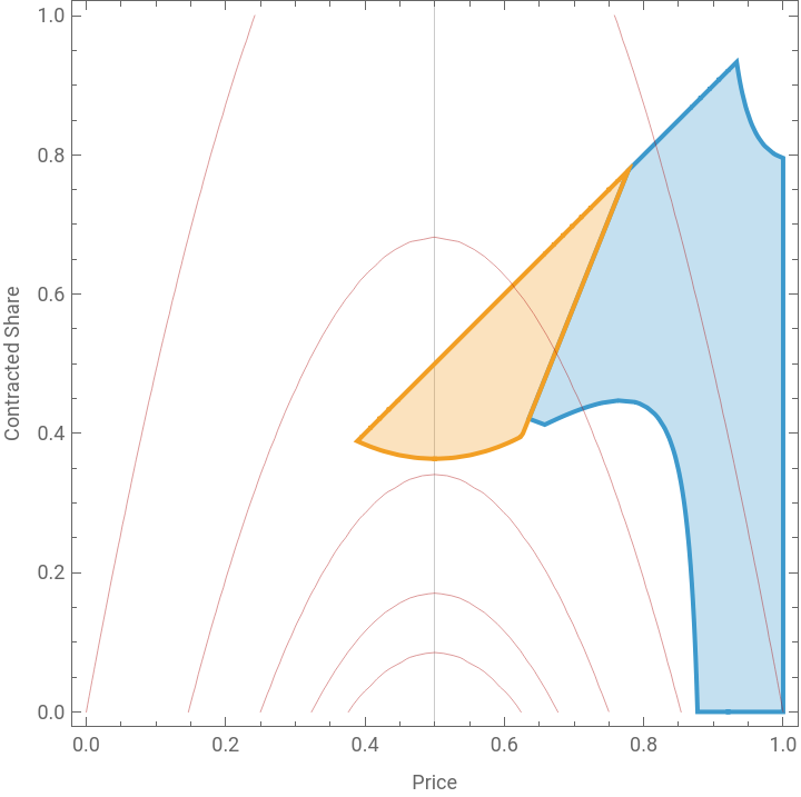
As described in the paper, the “blue region” in the figure above corresponds to price--contracting share pairs for equilibria in which the optimal deviation involves offering the equilibrium price; the “yellow region” corresponds to price--contracting share pairs for equilibria in which the optimal deviation involves offering a strictly higher price than the equilibrium price. We put a gridline at a price of .5 since that is the monopsony price; no lower price can be part of a profit-maximizing equilibrium.
Characterizing the Same-Price Deviation Equilibria
Characterizing the Same-Price Deviation Equilibria
Characterizing the No-Contracting Equilibrium
Characterizing the No-Contracting Equilibrium
We next find the price associated with the no-contracting equilibrium, i.e., the lowest price in the blue region for which the contracting share is 0. This is the price given in the high differentiation branch of the expression for the optimal price--contracting share pair in Theorem 3.
In[]:=
SolveCollusiveProfit[p,0,φ,ρ]==DeviatorProfit[p,0,φ,ρ],p;NoContractingPrice[δ_,φ_,ρ_]:=Evaluate[Nice[p/.%[[2]]]];NoContractingPrice[δ,φ,ρ]
φ
1-δ
Out[]=
-1+δ+ρ+δρ(-1+φ)+φ-ρφ
-1+δ+φ
Differentation Necessary for Perfect Collusion
Differentation Necessary for Perfect Collusion
We next solve for the differentiation at which it to possible to sustain the monopsony price with 0 contracting, that is the lowest differentiation. This corresponds to the upper bound for differentiation in Theorem 3.
In[]:=
NiceSolveNoContractingPrice[δ,φ,ρ]==,ρ;DifferentiationThresholdForPerfectCollusion[δ_,φ_]:=Evaluate[ρ/.%[[1]]];DifferentiationThresholdForPerfectCollusion[δ,φ]
1
2
Out[]=
-
-1+δ+φ
2(-1+δ)(-1+φ)
Minimal Contracting Share for Same-Price Deviations
Minimal Contracting Share for Same-Price Deviations
We now calculate the lowest contracting share to support a given price when the optimal deviation is to offer the same price as the collusive price while driving the residual supply to other long-lived firms to 0 (through increased aggressiveness). These are the price--contracting share pairs represented by the boundary of the blue region.
In[]:=
SolveCollusiveProfit[p,c,φ,ρ]==DeviatorProfit[p,c,φ,ρ],c;MinimalContractingShareBlueRegion[p_,δ_,φ_,ρ_]:=Evaluate[Nice[c/.%[[1]]]];MinimalContractingShareBlueRegion[p,δ,φ,ρ]
φ
1-δ
Out[]=
p(-1+δ)(-1+p+ρ)+p(-1+p+ρ-δρ)φ
(-1+φ)(-((-1+δ)(-1+p+ρ))+δρφ)
The High Differentiation Regime
The High Differentiation Regime
When differentiation is high enough, the most-profitable monopsony pricing equilibrium must occur in the blue region. To find the differentiation at which this is the case, we first determine, for any differentiation, the price at which the deviator’s unconstrained deviation price corresponds to exactly the proposed equilibrium price---that is, the price corresponding to the intersection of the blue and yellow boundaries in Figure 7.
In[]:=
Solve[UnconstrainedDeviationPrice[MinimalContractingShareBlueRegion[p,δ,φ,ρ],φ,ρ]==p,p];TransitionPrice[δ_,φ_,ρ_]:=Evaluate[Nice[p/.%[[1]]]];TransitionPrice[δ,φ,ρ]
Out[]=
-2+2ρ+2δ(1+ρ(-1+φ))+-1+
1+4ρ(-1+δ+ρ+δρ(-1+φ))
φ2(-1+δ-φ)
We also calculate at what differentiation the transition price becomes the monopsony price. At any higher differentiation, we need only consider the blue region.
In[]:=
NiceSolveTransitionPrice[δ,φ,ρ]==,ρ;DifferentiationWhereMonopsonyPriceIsTransitionPrice[δ_,φ_]:=Evaluate[Nice[ρ/.%[[2]]]];DifferentiationWhereMonopsonyPriceIsTransitionPrice[δ,φ]
1
2

Out[]=
-1+δ+φ-δφ+φ
δ-δφ
2(1+δ(-1+φ))(-1+φ)
Finally, we show that the no-contracting equilibrium is the most-profitable equilibrium at any differentiation above this threshold.
In[]:=
AbsoluteTimingFindInstanceCollusiveProfit[p,MinimalContractingShareBlueRegion[p,δ,φ,ρ],φ,ρ]>CollusiveProfit[NoContractingPrice[δ,φ,ρ],0,φ,ρ]&&And@@ParameterRestrictions&&DifferentiationWhereMonopsonyPriceIsTransitionPrice[δ,φ]<=ρ<=DifferentiationThresholdForPerfectCollusion[δ,φ]&&δ<=&&<=p<=NoContractingPrice[δ,φ,ρ],{p,δ,φ,ρ}
2
(1-φ)
1
2
The Low-Differentiation Regime
The Low-Differentiation Regime
Henceforth, we assume differentiation is low enough that, for the most - profitable monopsony pricing equilibrium, the optimal deviation is to a strictly higher price, i . e, the yellow region is the relevant region for the monopsony price of 0.5 .
Characterizing the Monopsony Pricing Point
Characterizing the Monopsony Pricing Point
We first solve for the smallest contracting share such for a monopsony pricing equilibrium, i.e., the lowest point in the yellow region. This is the contracting share given in the low differentiation branch of the expression for the optimal price--contracting share pair in Theorem 3.
We also characterize the lowest discount rate at which the monopsony price can be supported; this corresponds the lower bound on the discount rate in Theorem 3.
Characterizing the Possibly Optimal, Critical Point Price--Contracting Share Pairs
Characterizing the Possibly Optimal, Critical Point Price--Contracting Share Pairs
Next, we find the candidates for the extremal profit points in the blue region. Any such point must be on the boundary---as otherwise we could reduce the contracting share, keep the same price, and thus increase profits---and must either be the lowest-price point on the boundary---i.e., the transition price---or be a critical point---i.e., a point at which the derivative of the profits along the boundary of the blue region is 0.
We find the critical points by taking the derivative along the boundary of the blue region and setting it to 0; there are three solutions to this, which we call Candidate Prices #1-#3. Note that, due to how Mathematica solves cubics, Candidate Price #1 jumps when we go from 3 to 1 real roots; in particular, what was Candidate Price #3 when are three real roots becomes Candidate Price #1 when there is one real root. (Note how brown becomes red on the graph in the next section.)
We find the critical points by taking the derivative along the boundary of the blue region and setting it to 0; there are three solutions to this, which we call Candidate Prices #1-#3. Note that, due to how Mathematica solves cubics, Candidate Price #1 jumps when we go from 3 to 1 real roots; in particular, what was Candidate Price #3 when are three real roots becomes Candidate Price #1 when there is one real root. (Note how brown becomes red on the graph in the next section.)
We now plot how profits change with price along the boundary of the blue region; the yellow line is the profits of the monopsony pricing equilibrium (assuming it is in the yellow region), the dotted grid lines are at the monopsony price and the no-contracting price, the green dashed line is at the transition price, and the purple dashed lines are at the Candidate Prices.
Note that we have three roots only for some parameter values---in particular, a low enough differentiation.
The Non-Optimality of the Transition-Point Equilibrium
The Non-Optimality of the Transition-Point Equilibrium
We now show that the monopsony pricing equilibrium is always superior to the transition point equilibrium in the low differentiation regime. This follows from the fact that the monopsony pricing contracted share is always less than the contracted share of the transition point equilibrium (and the price is weakly higher--- and thus less profitable ceteris paribus---at the transition equilibrium as well).
The Non-Optimality of Candidate Price #1
The Non-Optimality of Candidate Price #1
We first show that Candidate Price #1 is only greater than 1/2 when differentiation is high enough. Is Either Irrelevant or Delivers Lower Profits than the No Contracting Equilibrium
For any lower differentiation, Candidate Price #1 is irrelevant as it has a lower price than the monopsony-pricing equilibrium:
For any higher differentiation, when Candidate Price #1 is greater than the monopsony price, the no-contracting equilibrium always deliver higher profits than Candidate Price #1.
The Non-Optimality of Candidate Price #2
The Non-Optimality of Candidate Price #2
We now check that when Candidate Price #2 is relevant, i.e., it is less than the no-contracting price, the slope of the profit function at the no contracting price is positive; thus, since Candidate Price #2 is the first critical point to the left of the no-contracting price, it must deliver lower profits than the no-contracting equilibrium.
The Non-Optimality of Candidate Price #3
The Non-Optimality of Candidate Price #3
We now show that the Candidate Price #3 is never relevant, i.e., that it is always greater than the no contracting price. To do this, we first check that when all the roots are real Candidate Price #3 is always greater than the no-contracting price.
When differentiation is high enough so that there is only one real root, Candidate Price #3 is relabeled by Mathematica as one of the imaginary roots, and Candidate Price #1 remains the real root. Thus, we finish by checking that “Candidate Price #1” is always greater than the no contracting price at such differentiations.
Uniqueness of the Cutoff Differentiation
Uniqueness of the Cutoff Differentiation
Finally, we prove that the profits of the monopsony-pricing equilibrium are decreasing in differentiation and the profits of the no-contracting equilibrium are increasing in differentiation. First, we show that the profits of the monopsony-pricing equilibrium are non-increasing in differentiation.
Next, we show that the profits of the no-contracting equilibrium are increasing in differentiation.
CITE THIS NOTEBOOK
CITE THIS NOTEBOOK
Facilitating Collusion with Spot-Price Contracting
by John Hatfield
Wolfram Community, STAFF PICKS, August 10, 2023
https://community.wolfram.com/groups/-/m/t/2987807
by John Hatfield
Wolfram Community, STAFF PICKS, August 10, 2023
https://community.wolfram.com/groups/-/m/t/2987807