Wolfram Cloud Document

CITE THIS NOTEBOOK: Extracting linguistic relations fr. word embeddings&language models by Cayden Pierce. Wolfram Community JUL 2022.

We wish to understand the meaning encoded by natural language in a symbolic and computable way, but natural language is complex and difficult to represent as such, and thus we attempt to understand linguistic relationships by exploring their representation within word embedding models and language models. While previous and SOTA approaches to natural language understanding (NLU) focus on end-to-end learning systems which generate a pipeline of encodings that are not explored or understood by the humans creating them, we directly analyzed and explored natural language embedding space as a step towards understanding natural language as a symbolic, self-referential system. We went beyond previous SOTA in human interpretability of word embedding space through discovery of representation of grammar, abstract word classes, notions of abstraction, global relationships between words, etc., and began the development of algorithms for combining these findings to create usable systems for tasks such as bogus grammar detection, synonym and antonym classification, same-class terms generation, and word definition checking/generation. Future work will take advantage of these discoveries to translate natural language into a symbolic language that is simultaneously human- and machine-understandable, creating the possibility for conversational language that is unambiguous, machine interpretable, and able to act on data and objects of the real world.

Word Relationships as Translation Vectors

Differences between words/concepts can be represented as translation vectors in word embedding space, these translation vectors are defined as the difference (subtraction) between the word embeddings of the two words being compared. The translation vector represents a direction and magnitude one must travel to get from one word embedding to another.

Be sure to run the code in the two sections below, everything else in this notebook relies on them:

Loading Word Embedding Models


Loading Data


SOTA - (king - man + woman = queen)

The state of the art interpretation of human interpretability of word embedding model spaces is centered around a geometric understanding of the space, whereby addition and subtraction of words can yield new words. The classic formulation of this concept is represented as (king - man + woman = queen):

The classic word embedding equation:

In[]:=

Nearest[word2vecGl,word2vecGl["king"]-word2vecGl["man"]+word2vecGl["woman"],8]

Out[]=

{king,queen,monarch,mother,princess,daughter,elizabeth,throne}

Notice above that “king” is still the first result. This is surprising to some, but it’s how the algorithm actually works! The usual implementation of word analogies with word embedding models excludes the input word from the output of the algorithm, but we give the raw output above to demonstrate this fact.

Generalizing Word Meaning Translations

(king - man + woman = queen) is a way to represent the algebraic relationships between words in embedding space. To generalize this concept, one can extract a translation vector and starting point from the above equation in the form of (word + translation = translated_word). For example, (woman - man) is our translation vector and (king) is the starting word. The given translation vector can now be considered as a generic translation from the masculine representation of a concept to the feminine, and thus applied to other words, as below.

Generate gender translation vector and apply to example word (in direction of female to male):

In[]:=

conversion={{"he","she"},{"man","woman"}};ConceptNetTransitions[words_List,modelAssoc_]:=Rule[StringJoin[#[[1]],", ",#[[2]]],Flatten[modelAssoc[#[[1]]]-modelAssoc[#[[2]]]]]&/@words;converterTrans=Mean[Values[Association[ConceptNetTransitions[conversion,word2vecGl]]]];

In[]:=

Nearest[word2vecGl,word2vecGl["waitress"]+2.2*converterTrans,8]

Out[]=

{bartender,man,waiter,beefy,burly,busboy,janitor,guy}

In[]:=

Nearest[word2vecGl,word2vecGl["actress"]+2.2*converterTrans,8]

Out[]=

{actor,man,starred,starring,he,played,movie,mr.}

Decomposing relationship - word relationship basis vectors

Word embedding space is high dimensional. The word2vec models in use here are ConceptNet NumberBath and GloVe, which are both 300 dimensions. In this type of space, it’s a common operation to reduce the dimensionality of a subset of data points to the principal components in order to consider only a subspace of the word embedding manifold. The principal components form basis vectors in which the variance of the data subset is maximized.

Analogously, one can form basis vectors using arbitrary orthogonal bases. In latent space, where direction corresponds to change in meaning, one could choose a translation vector as the principal vector in a basis, and thus a dimension can correspond to some predetermined meaning space gradient - like small tocomm large, young to old, poor to rich, etc.

Inspired by this idea, we form pairs of numbers {w1_n, w2_n} which are antonyms of each other, transform them into vector pair {e1_n, e2_n} with w2v(w_n), subtract them (e_1 - e_2), and normalize all elements to form a list, ϕ, of length n populated by word translation vectors of size w2v_dimensions. Then, a pair of words is manually chosen whose difference one wishes to assess. This chosen word pair is embedded and the difference between the embeddings is taken to form another word translation vector η. List ϕ is then searched for the nearest occurrences of η, and the results represent translations in meaning space corresponding to the input word pair. These translations can be thought of as the basis vectors for our input words, chose from ϕ to maximize variance, and thus serve as a description of the most important relationships between any pair of words.

Generate sets of antonym pairs as word relationship decomposition, exploring the strongest differences between two given words:

In[]:=

antoSet=Normal[{#lemma,StringSplit[#antonyms,"|"|";"][[1]]}&/@RandomSample[antonymsData,Length[antonymsData]-1]];commonAntonyms=If[MemberQ[Normal[commonEnglishWords[All,"Word"]],#[[1]]|#[[2]]],#,Nothing]&/@antoSet;

In[]:=

commonAntonymsVectors=Apply[Rule[#1<>":"<>#2,{word2vecCn[#1],word2vecCn[#2]}]&,commonAntonyms,2];

In[]:=

commonAntonymsVectorsNew=Select[commonAntonymsVectors,((Length[Values[#][[1]]]==300)&&(Length[Values[#][[2]]]==300))&];

In[]:=

commonAntonymsVectorsTvsNormalized=Rule[Keys[#],Normalize[Subtract[Values[#][[1]],Values[#][[2]]]]]&/@commonAntonymsVectorsNew;

In[]:=

PrincipalRelations[word1_String,word2_String]:=Nearest[Association[commonAntonymsVectorsTvsNormalized],(word2vecCn[word1]-word2vecCn[word2]),10]

Decompositions of word relations into canonical translation vectors

In[]:=

PrincipalRelations["kitten","cat"]

Out[]=

{little:large,small:large,birth:death,junior:senior,nonage:majority,small:big,nascency:death,littler:large,inexperienced:experienced,minor:major}

In[]:=

PrincipalRelations["beggar","player"]

Out[]=

{worthless:valuable,powerless:powerful,unskilled:skilled,weak:strong,volunteer:draftee,untalented:talented,talentless:talented,incapable:capable,disadvantaged:advantage,voluntary:draftee}

In[]:=

PrincipalRelations["summer","winter"]

Out[]=

{hot:cold,heat:coldness,boiling:freeze,unrealistic:realistic,boil:freeze,diffused:hard,boiled:freeze,liberal:conservative,unwind:wind,flunk:pass}

In[]:=

PrincipalRelations["republican","democrat"]

Out[]=

{conservative:liberal,armed:unarmed,military personnel:civilian,rapidly:slowly,superficial:profound,aggressive:unaggressive,salty:fresh,unborn:born,forward:backward,regressive:progressive}

The final relationship decomposition above alludes to how we might extract cultural beliefs and biases from word embedding models.

General Distance and Translation Statistics

What types of general similarities exist with certain classes of word relationships, and how do class of word relationships differ from each other?

Algorithm

Form pairs of words whose relationships follow a given property, thus we have a list of pairs {{w1_1,w2_1},...{w1_n, w2_n}} of length n whereby w1 and w2 are related by being synonyms, antonyms, or randomly chosen words.

Transform pairs of words into pairs of vectors by obtaining the word embedding for each word pair as {e1_n = w2t(w1_n), e2_n = w2t(w2_n)}

Generate n pairs of random vectors.

For all sets generated above, compute the difference between two pairs, yielding a list of length n of translation vectors in word embedding latent space. Compute the distance between each pair of vectors, and finally plot a histogram of the distribution of these distances.

Synonyms

In[]:=

synoSet=Normal[{#lemma,StringSplit[#synonyms,"|"|";"][[1]]}&/@RandomSample[synonymsData,20000]];

In[]:=

commonSynonyms=If[MemberQ[Normal[commonEnglishWords[All,"Word"]],#[[1]]|#[[2]]],#,Nothing]&/@synoSet;

In[]:=

commonSynonymsVectors=Apply[Rule[StringJoin[ToString[#1],":",ToString[#2]],{word2vecCn[#1],word2vecCn[#2]}]&,commonSynonyms,2];

In[]:=

commonSynonymsVectorsClean=Select[commonSynonymsVectors,((Length[Values[#][[1]]]==300)&&(Length[Values[#][[2]]]==300))&];

In[]:=

synoDistances=Apply[EuclideanDistance,Values[commonSynonymsVectorsClean],1];

Random word pairs

In[]:=

randomWordPairs=Transpose[{RandomSample[wordsCn,2276],RandomSample[wordsCn,2276]}];

In[]:=

randomWordPairsVectors=Apply[Rule[StringJoin[ToString[#1],ToString[#2]],{word2vecCn[#1],word2vecCn[#2]}]&,randomWordPairs,2];

In[]:=

randomWordPairsDistances=Apply[EuclideanDistance,Values[randomWordPairsVectors],1];

Antonyms

In[]:=

commonAntonyms=If[MemberQ[Normal[commonEnglishWords[All,"Word"]],#[[1]]|#[[2]]],#,Nothing]&/@antoSet;

In[]:=

commonAntonymsVectors=Apply[Rule[StringJoin[ToString[#1],":",ToString[#2]],{word2vecCn[#1],word2vecCn[#2]}]&,commonAntonyms,2];

In[]:=

commonAntonymsVectorsClean=Select[commonAntonymsVectors,((Length[Values[#][[1]]]==300)&&(Length[Values[#][[2]]]==300))&];

In[]:=

antonymsDistances=Apply[EuclideanDistance,Values[commonAntonymsVectorsClean],1];

Random Vector Pairs (not token embeddings)

In[]:=

randomVec[r_,d_]:=r*Normalize@RandomVariate[NormalDistribution[],d]

In[]:=

randomVectorPairs=Transpose[{Table[randomVec[1,300],2276],Table[randomVec[1,300],2276]}];

In[]:=

randomVectorPairsDistances=Apply[EuclideanDistance,randomVectorPairs,1];

Click the image below to flip between the plots:

In[]:=

FlipView[{Histogram[synoDistances,PlotLabel->"Synonyms Distances",ImageSizeLarge],Histogram[antonymsDistances,PlotLabel->"Antonyms Distances",ImageSizeLarge],Histogram[randomWordPairsDistances,PlotLabel->"Random Word Embedding Distances",ImageSizeLarge],Histogram[randomVectorPairsDistances,PlotLabel->"Random Vector Distances",ImageSizeLarge]}]

Out[]=

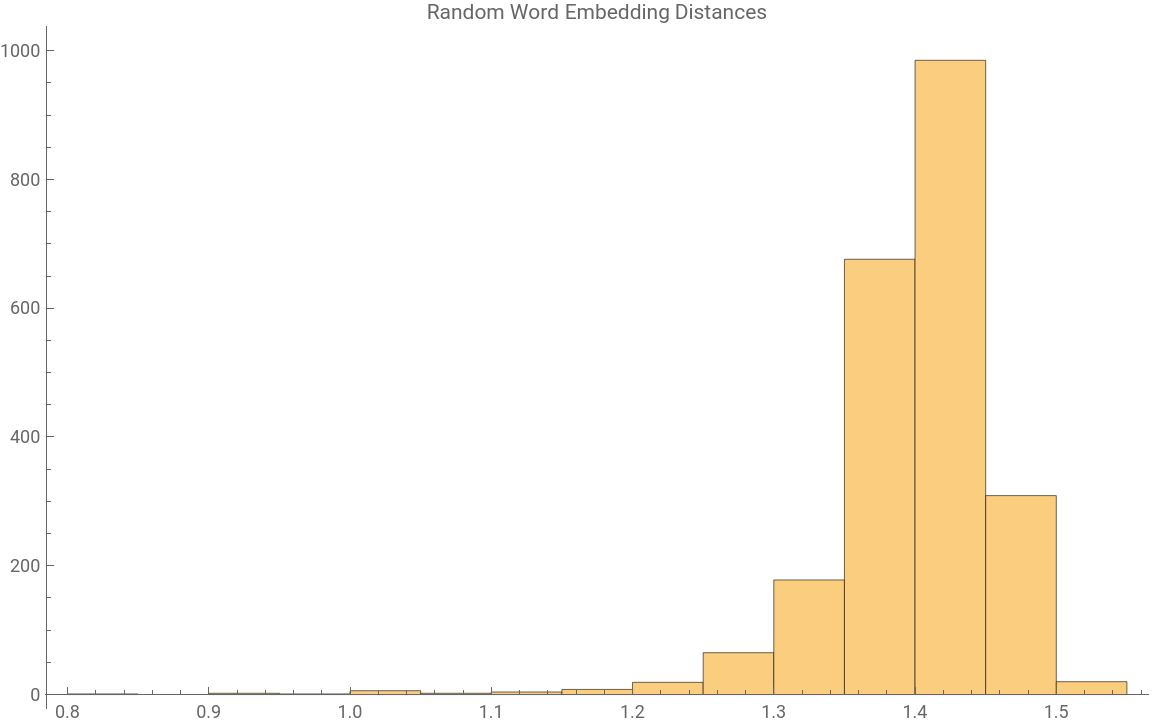
These results show that synonyms, antonyms, random word pairs, and pairs of randomly generated points all have different characteristic translation vector (difference) distribution plots. Synonym translation vectors are always short, antonyms are short but longer than synonyms, random word pairs translation vectors chosen from the word2vec vocabulary have a peaked distribution centered at ~1.4, and randomly chosen point pairs translation vectors follow a normal distribution with a mean of ~1.4.

Visualizing the Latent Space

Word embeddings are the result of training an unsupervised, single hidden layer neural network either to predict a masked word given context (continuous bag of words method, CBOW) or by predicting the context given a certain word (skipgram). The input dimension to this system is normally the size of the word embedding system vocabulary (one hot encoded) and the representation (latent space) dimensionality is the number of neurons in the the single hidden layer.

A network which utilized the full dimensionality of the embedding space would yield word embeddings which were uniformly distributed across the meaning space and would look similar to the below:

Uniformly distributed unit vectors in 300 dimensions form uniform sampling of a 300 dimensional hypersphere, projected in 2D:

In[]:=

randomVec[r_,d_]:=r*Normalize@RandomVariate[UniformDistribution[],d]

However, most word embedding systems don’t use techniques to force an even distribution of word embeddings throughout the embedding space, and thus their latent space representations form interesting clusters and contain most variance in a limited set of principal components:

Random sample of ConceptNet Numberbatch word embedding latent space, projected in 2D:

Random sample of GloVe word embedding latent space, projected in 2D:

Walks Through Meaning Space

After observing the geometric relationships between words discussed above, one might wonder what other words and concepts lie along the path from one word to another? One might explore this question in a number of ways, such as taking the translation vector between two words and making incremental steps along the path, at each point finding all words which lie nearest to that location in embedding space.

Straight Walk

tv is the translation vector between word embeddings e_1 and e_2, corresponding to words w_1 and w_2, respectively.

A word walk is defined as the nearest words in latent space along a series of discrete steps along tv.

steps(i) = e_1 + (tv/i_max*i)

state(i) = Nearest(w2v, steps(i))

Straight walk visualized in graph form:

Word Class Subspaces

Clustering word embedding spaces with traditional clustering techniques (e.g. K-means) has classically been considered a poor approach to divide the word embedding space in a meaningful way. This largely has to do with the overlap/overloading of different concepts, classes, and translations in meaning space, such that looking at just the nearest words yields many words which seem largely unrelated to the class under investigation.

This limitation is evident when one wishes to look for all words that belong to a given class. A naive approach would be to look for all words near the mean of a subset of words that define that class. However, due to the issue described above, this does not yield only words which belong to the class under test. For example, if one simply takes all of the words that are near the mean of a small group of words which belong to the class “animal”, this yield many words that would not be considered to belong to the class “animal”:

We hypothesize that a class of words does have a unique relation, but this relation exists in a subspace of the word embedding space, such that simple distance metrics do not capture this relation.

To discover if this is the case, we specify a class of words (e.g. all names of animals) C, manually generate examples of those words, and get the volume of the simplex formed by each word in an n-dimensional hypersphere surrounding the centroid/mean of the word embeddings of C (C_e). One would expect the simplices of words in the target class to have smaller volumes than words of a separate class, as in-class words should lie in the same subspace plane as those in C_e, and non-members will lie outside of that subspace, and thus creating a larger volume. Thus, we cluster the simplex volumes into two groups and take the group with the smaller average value as members of the target class.

◼

Define representative sample tokens of class (e.g. {bird, lion, tiger, wolf, dolphin}), called set C

◼

Embed members of set C to form set C_e, find 1000 nearest words to the mean of C_e, this 1000 nearest words forms set D

◼

Define 1000 simplices whose vertices are the members of set C_e concatenated with the embedding of a word in D. Compute the volume of each simplex using the Cayley-Menger Determinant: V_j^2(S)=((-1)^(j+1))/(2^j(j!)^2)det(B^^)1

◼

Cluster the resulting volumes into two groups. Whichever cluster has the smaller average volume is the group of words which represent the class under test.

Cayley-Menger Determinant (credit: Markus van Almsick)

Class subspace finding:

Demonstrate that simple nearest neighbour of class representatives does not work to define a class. One can see below that the words fetched are not members of the class “animal” despite being closest to animal examples in latent space.

We see that the simplex volume of our nearest words and example corpus show a clear separation - so we cluster.

The content below is all words that are near the mean of our example words, but clustering them based on simplex volume shows clear differentiation between the words words of the class specified and other words.

Thus, classes do exist within subspaces, and these can be found with a few class representative and simplex volumes.

Embedded Grammar

Word embeddings are considered very powerful in their ability to encode relationships between words, but it’s generally thought that there is little or no grammatical information embedded in these models.

We believe that this assumption is not accurate, as the distributional hypothesis should hold in terms of co-occurence of words and the proper grammatical word forms surrounding them, and thus word embeddings models should embed some grammatical information.

It was discovered that this is indeed the case, and can be seen by taking the inner product of two subsequent words in a phrase. When comparing grammatical and agrammatical phrases, the grammatical phrase has a larger inner product:

The exploration above indicates that two-word English phrases have a larger inner product than improper two-word English phrases.

This can be visualized intuitively by painting the background colors of word pairs with a color that represents the inner product value (red: low, green: high) :

Tying this all together, one can write a function that compares two sentences - one of proper English grammar form and another of improper grammar - and returns a relative rating of each sentence, where the sentence with the higher number is more grammatically correct than the other:

Linguistic Equations

One of the early goals of this project was the ability to create linguistic equations, equations in which the LHS represents a single word and the RHS represents the definition of that word or another expression which means the same thing. The first step to construct this type of object is the ability to understand and parse meaning from words and language.

Heretofore in this notebook, we have demonstrated various ways in which word meaning can be extracted, represented, and manipulated. For a single word linguistic equation, word embeddings may be enough, however, linguistic equations may include phrases or sentences that must be ascertained for meaning. An end-to-end learning approach would utilize sentence embeddings generated by transformer based models (e.g. BERT) and compare these sentence embeddings. In order to better understand how phrases and sentences are built up to generate meaning, we consider these word equations at the level of individual words.

Word1 = Translation + Word2

Let’s consider linguistic equations of the form

word == adjective + noun

for example:

“ostrich” == “flightless bird”

Which can be expressed as:

ω1 = ω2 + ϵ

Where ωn are nouns and ϵ is an adjective.

ωn can simply be represented by the word embedding of the given word. The adjective ϵ is some translation vector that the adjective imposes on the word. As such, we now need to represent an adjective as the translation vector it represents in word embedding space, and then add this to our ω2, and finally evaluate the distance between the LHS and RHS and determine the probability that the linguistic equation is valid.

To do so, we can parse out the adjective, retrieve its word embedding, and search through the dataset of antonym pair translation vectors (generated in previous sections). Upon finding the best match, we can define this as ϵ, add ϵ to ω2, and then assess the validity of the word equation based on the euclidean or cosine distance between the two sides of the linguistic equation.

Determine equality of linguistic equations of form word == adjective + noun:

While not always correct, the above rule based method of evaluating a specific form of word equations works quite well.

Abstract and Concrete Words

Abstract and concrete refers to a gradient or divide between entities, in which concrete entities are things that exist in the real world, often with physical instantiation, while abstract entities are more general concepts that might exist only as thoughts or ideas.

We aim to develop an “abstraction index”, a function which takes in a word and returns an abstraction score, as a float [0,1], where 0 is concrete (e.g. bathtub) and 1 is abstract (e.g. spirituality) or an analogous graph or tree which represents abstraction relationships between words. To do so, one must be able to ascertain differences between concrete and abstract words. Below, we explore a number of methods for assessing, out of two words, which is the more abstract, and then forming a vocabulary tree which is parsed to generate an ordering of words from concrete to abstract.

Distance of surrounding nearest words (failed)

Words which frequently occur in the same context will be close together in word embedding latent space, and conversely, words that don’t appear in the same context are further apart. With this in mind, one might conjecture that more abstract words (within a class of words in a certain subspace) would be positioned closer to other members of the class than a more concrete word, which is not able to replace other words in text. For example, “red” is a “color”, and “green” is a “color”, but “red” is not “green”, and this analogy continues for many words in the class. “color” is the abstract word here, and would be expected to have an average distance to the surrounding words in its class which is less than the average distance to surrounding word of “red” or “green”.

To explore this conjecture, we construct pairs of words, the first of which is abstract, and the second of which is concrete and could be abstractedly defined by the first word. Embed these words and look at the n nearest words to each given embedding. Take the distances between these nearest words and the embedding of the given word, and assess the differences distribution, comparing that of concrete words with that of abstract words.

Get embeddings of word pairs

Find nearest words to each manually input word

Turn nearest words into embeddings

Get distances between input word and nearest words.

Abstract on left, concrete on right:

Assessing the distributions above, it appears that our hypothesis does not hold, as there is not an obvious mean offset between abstract and concrete words in the comparison histogram plots.

Translation vector to nearest words direction (failed)

It seems abstraction is not captured in average surrounding word differences, but perhaps there is a quantitative difference in the direction of how words are distributed in the space based on their abstraction. One can consider all of the translation vectors between a specific class member and all other members of that class, and take the mean of this vector as the average class pointing direction for a given word in a given class. If this vector is different for abstract words and concrete words, it can be used as a metric to develop an abstraction index. To test this, we extract a subspace class of “animal” and assess if average class pointing direction vectors are different for abstract and concrete words.

First, we get the subclass of “animal” words, as explain in the “Subspace Classes” section above:

Again, we don’t see a clear differentiation between abstract and concrete words. One could continue down this path, and the intuition we’ve built up from other experiments makes one suspect that information about abstraction is probably embedded in the word embedding space in some way, shape, or form. However, let’s explore some different approaches to extract abstraction from statistical word systems.

Transformer Language Model Prompts - Abstraction as “to be”

Abstraction can often represented as a “to be” relationship. A “labrador” is a “dog”, which is a “canis”, which is an “animal”, which is a “life form”. This “to be” chain of membership often exactly follows the path from concrete to abstraction, as:

abstraction(“labrador”) < abstraction(“dog”) < abstraction(“canis”) < abstraction(“animal”) < abstraction(“life form”)

So, how can we take advantage of this relationship in order to rate words as more or less abstract than other words?

Transformer based language models are powerful learning systems for seq2seq (sequence to sequence) transformation learning problems. The Wolfram Language has a number of built in language models pre-trained for various tasks, such as text generation, whereby the system input is a natural language string and the output is natural language continuation of that text.

Combining these, one can define a system whereby a phrase that defines a possible “to be” abstraction relationship is input to a transformer model (such as GPT-2), and the first predicted output distribution is considered. For example, given the terms “cat” and “animal”, one can assess which sentence is more likely: “cat is an animal” or “animal is a cat”, and based on the result ascertain whether one of these words is a subset of the other.

Now we have an abstract to concrete assessment function, we need to generate some representation of words in the language in a structure that shows the abstraction relationships/ordering of words. A first step towards this is forming a set of directed edges where the direction points from in the direction from abstract to concrete.

One can see above a graph structure with directed edges that point from more concrete words to more abstract words. This creates a tree-like structure that represents an abstraction hierarchy in the English language.

Weaknesses of this approach are caused largely by ambiguity of the English language. While the “to be” relationship holds in many cases, it doesn’t always hold. For example, one might say “the car is red”, which defines a property relationship, not a class-subset relation, and thus does not represent abstraction, as “red” can be a property of “car”, but is not an abstraction of “car”?

Conclusion

A series of questions concerning how word embeddings and language models represent meaning, relationships, grammar, etc. in latent space were proposed and explored. The multiple discoveries and examples of word embeddings and language model behaviour and meaning representation presented in this notebook can lead one to a better intuitive understanding of NLP systems, which can be used to improve systems of the future. Further, work here on decomposition of word differences and word definition/generation is a step towards symbolic understanding, interpretation, and generation of language. Future work will take advantage of these discoveries to translate natural language into a symbolic language which encodes meaning yet is simultaneously human- and machine-understandable, creating the possibility for conversational language that is unambiguous, machine interpretable, and able to act on data and objects of the real world.

Keywords

◼

Natural Language Processing (NLP)

◼

Natural Language Understanding (NLU)

◼

Word Embeddings

◼

Word relations

◼

Word meaning

◼

Language Models

◼

Latent Space

◼

Word equations, linguistic equations

◼

Grammar

◼

Artificial Intelligence (AI)

◼

Explainable Artificial Intelligence (XAI)

Acknowledgment

I’d like to thank Markus van Almsick, my project mentor, for extensive help, ideas, mentorship, and fun conversations throughout the project. Thanks to Stephen Wolfram for initial definition of the project, advice during the summer program, and for running the Wolfram Summer School 2022. Thanks also to Mads, Emily, Danielle, and everyone else involved in running Wolfram Summer School 2022.