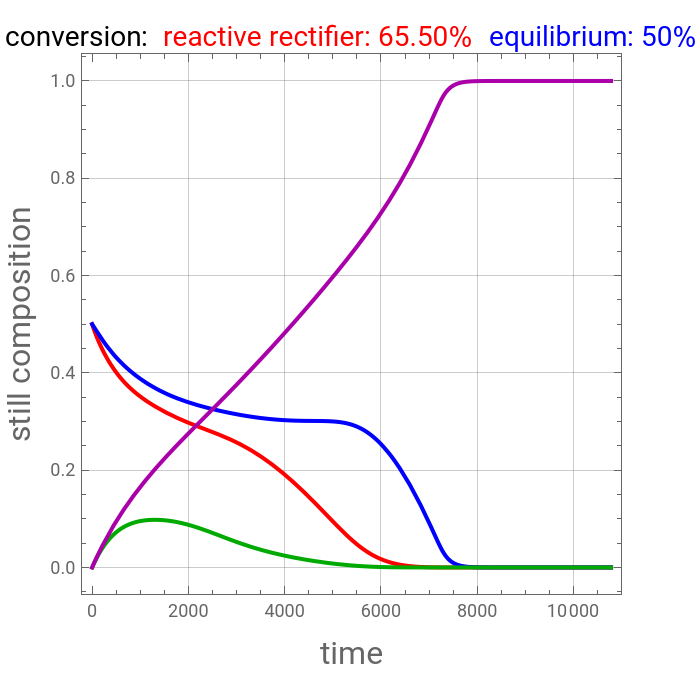
Consider an ideal quaternary mixture subject to an equilibrium-limited chemical reaction . The relative volatilities are taken as =4, =3, =7, and =1. The products and appear as the highest and lowest boiling point components of this quaternary mixture. An equimolar mixture of and is initially fed to a reactive rectifier. For simplicity, assume that the reaction takes place only in the still. This notebook plots the distillate and still compositions versus time for two values of the Damköhler number (see parameter , which varies between 0 and 1. We take the reflux ratio , the equilibrium constant =1 (used in the rate expression as follows: ), and the number of nonreactive stages in the rectifier . Compositions of components , , , and are plotted in red, blue, green, and magenta, respectively.
A+B⇌C+D
α
AD
α
BD
α
CD
α
DD
C
D
A
B
Da
u=Da/(1+Da)
R=10
K
eq
r=k-
C
A
C
B
C
C
C
D
K
eq
N=13
A
B
C
D
It is clear from the last plot that when is high, one gets pure and pure and a minor intermediate fraction containing mainly unreacted and . Thus it is possible to drive the reaction conversion to very high values to recover the pure products, components and . One can try a situation where and no products are formed. As expected, increasing favors more production of and . The conversions achieved by combining separation and reaction in one unit operation are far superior to the equilibrium value achieved without separation. These two conversions are reported as percentages in the still and distillate composition plots.
Da
C
D
A
B
C
D
Da=0
K
eq
C
D
In[]:=
V=1;F=1000;HP=1;HD=2;xA0=0.5;a14=4;a24=3;a34=7;Ntot=15;R=10;Keq=1;Da=u/(1-u);Dif=V/(R+1);L=V-Dif;
In[]:=
(*compositionofDandvapour-liquidequilibrium(constantrelativevolatilities)*)x4[i_][t_]:=1-x1[i][t]-x2[i][t]-x3[i][t];den[i_][t_]:=a14x1[i][t]+a24x2[i][t]+a34x3[i][t]+x4[i][t];y1[i_][t_]:=a14x1[i][t]/den[i][t];y2[i_][t_]:=a24x2[i][t]/den[i][t];y3[i_][t_]:=a34x3[i][t]/den[i][t];rate[i_][t_]:=x1[i][t]x2[i][t]-x3[i][t]x4[i][t]/Keq;xs={x1,x2,x3};ys={y1,y2,y3};sgn={-1,-1,+1};(*AandBconsumed,Cproduced*)
In[]:=
(*traysi=2..Ntot-1*)trays=Flatten@Table[HPD[xs[[k]][i][t],t]==L(xs[[k]][i-1][t]-xs[[k]][i][t])+V(ys[[k]][i+1][t]-ys[[k]][i][t]),{k,3},{i,2,Ntot-1}];(*condenser,stage1*)cond=Table[HDD[xs[[k]][1][t],t]==Vys[[k]][2][t]-(L+Dif)xs[[k]][1][t],{k,3}];(*still,stageNtot,withreaction*)(*reactionrateproportionaltostillholdup*)still=Table[D[M1[t]xs[[k]][Ntot][t],t]==-Vys[[k]][Ntot][t]+Lxs[[k]][Ntot-1][t]+sgn[[k]]DaL(M1[t]/F)rate[Ntot][t],{k,3}];eqM=D[M1[t],t]==-Dif;init=Join[Flatten@Table[xs[[k]][i][0]=={xA0,xA0,0}[[k]],{k,3},{i,Ntot}],{M1[0]==F}];funct=Append[Flatten@Table[xs[[k]][i][t],{k,3},{i,Ntot}],M1[t]];(*M1reaches0att=F/Dif,wherethebalancesbecomesingular:stopslightlybefore*)tEnd=0.98F/Dif;
Case 1 : Damköhler number =1 (i.e., )
Da
u=Da/(1+Da)=0.5
In[]:=
u=0.5;
In[]:=
sol=Quiet@NDSolve[Join[trays,cond,still,{eqM},init],funct,{t,0,tEnd},Method->{"EquationSimplification"->"Residual"},AccuracyGoal->5];
In[]:=
(*Aconsumedbyreaction(integralofthestillreactionterm)dividedbytheAinitiallypresentinstill,traysandcondenser*)consumed=NIntegrate[Evaluate[DaL(M1[t]/F)rate[Ntot][t]/.sol],{t,0,tEnd}];C0=xA0(F+(Ntot-2)HP+HD);conv=100consumed/C0;
In[]:=
(*equilibriumconversionofAforanequimolarA/Bfeed:Keq=xi^2/(0.5-xi)^2⇒conversion=2xi/1=s/(1+s)withs=Sqrt[Keq]*)s=Sqrt[Keq];eqConv=100s/(1+s);
In[]:=
stageplot=Ntot;(*still*)
In[]:=
p1=Plot[Evaluate[{x1[stageplot][t],x2[stageplot][t],x3[stageplot][t],x4[stageplot][t]}/.sol],{t,0,tEnd},PlotRange->All,Frame->True,GridLines->Automatic,AspectRatio->1,ImageSize->350{1,1},FrameLabel->{Style["time",16],Style["still composition",16]},PlotStyle->{{Red,Thick},{Blue,Thick},{Darker@Green,Thick},{Darker@Magenta,Thick}},PlotLabel->Row[{Style["conversion:",14,Black]," ",Style[Row[{"reactive rectifier: ",NumberForm[First@conv,{3,2}],"%"}],14,Red]," ",Style[Row[{"equilibrium: ",NumberForm[eqConv,{3,2}],"%"}],14,Blue]}]]
Out[]=
In[]:=
stageplot=1;(*distillatestream*)
In[]:=
p2=Plot[Evaluate[{x1[stageplot][t],x2[stageplot][t],x3[stageplot][t],x4[stageplot][t]}/.sol],{t,0,tEnd},PlotRange->All,Frame->True,GridLines->Automatic,AspectRatio->1,ImageSize->350{1,1},FrameLabel->{Style["time",16],Style["distillate composition",16]},PlotStyle->{{Red,Thick},{Blue,Thick},{Darker@Green,Thick},{Darker@Magenta,Thick}},PlotLabel->Row[{Style["conversion:",14,Black]," ",Style[Row[{"reactive rectifier: ",NumberForm[First@conv,{3,2}],"%"}],14,Red]," ",Style[Row[{"equilibrium: ",NumberForm[eqConv,{3,2}],"%"}],14,Blue]}]]