Out[]=
We introduce a new space-filling curve, whose “-function” can be written with three symbols {-1,0,1} distinguishing between the edge vectors of a triangular lattice. The curve is quite similar to the original paper folding dragon curve. It could already have been discovered as early as 1999, perhaps earlier, but we have no evidence that it was. The purpose of this memo is to give a few clumsy definitions in support of a zany transformation theorem, which we previously speculated to exist, and also to give a few more definitions which mathematicians might find to be more useful for proof and analysis.
Shift operators & recursion depth
Shift operators & recursion depth
For a project at WSS2024, Thomas Adler and I needed to look for integer shift functions satisfying the inequality , when . Such bounded shifts are useful when constructing recursive functions, because they can help ensure absence of unbounded growth.
0≤S[n]<n
n∈
For example, here is a very simple LinearShift function:
In[]:=
LinearShift[_,_]=1;LinearShift[n_?Positive,a_?Positive]:=n-a
which allows the Fibonacci sequence to be written as follows:
In[]:=
Fib[0]=Fib[1]=1;Fib[n_]:=Fib[n]=Fib[LinearShift[n,1]]+Fib[LinearShift[n,2]];
In[]:=
Fib/@Range[0,10]
Out[]=
{1,1,2,3,5,8,13,21,34,55,89}
Considering that we’ve known this sequence for 100’s or even 1000’s of years, it’s nowadays difficult to get excited about unless it accompanies some sort of nature picture. Rather than that, let’s take the same functional form and substitute other shift functions, just to see what happens.
In[]:=
ClumsyShift[b_,op_:Plus][n_]:=FromDigits[Mod[op[IntegerDigits[n,b],1],b],b]
In[]:=
CycleShift[b_][n_]:=With[{digs=IntegerDigits[n,b]},FromDigits[Mod[digs-First[digs],b],b]]
Our divergent first idea, ClumsyShift, is the starting place, and its refined child, CycleShift, is closer to where the referees expect us to land. Both of these functions operate on digit strings by truncating most significant digits, but sometimes when , ClumsyShift may take as many as steps to reach leading zeroes.
b>2
b-1
Plugging this into the Fibonacci form, we find the Log function useful in reducing powers of two:
In[]:=
ClumsyRecurrence[0]=ClumsyRecurrence[1]=1;ClumsyRecurrence[n_]:=ClumsyRecurrence[n]=Plus[ClumsyRecurrence[ClumsyShift[2,Plus][n]],ClumsyRecurrence[ClumsyShift[2,Subtract][n]]]
In[]:=
Row[ListPlot[Log[2,ClumsyRecurrence/@Range[0,2^#-1]],ImageSize->300]&/@{5,10},Spacer[15]]
Out[]=
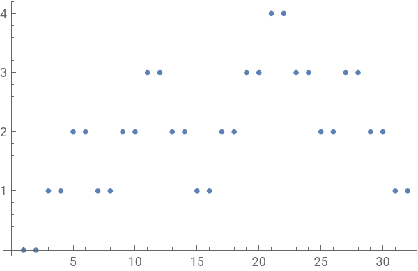

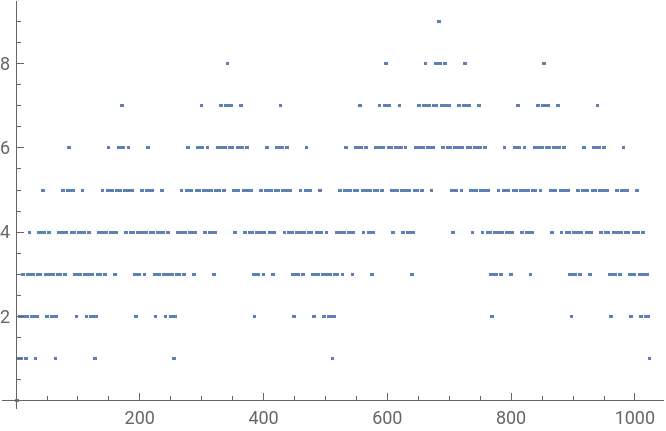
In[]:=
Log[2,ClumsyRecurrence/@Range[0,2^6-1]][[1;;-1;;2]]
Out[]=
{0,1,2,1,2,3,2,1,2,3,4,3,2,3,2,1,2,3,4,3,4,5,4,3,2,3,4,3,2,3,2,1}
This is quite strange to use both variants of ClumsyShift and Log, when it is also possible to get the same sequence just by defining the RecursionDepth, and evaluating it for CycleShift:
In[]:=
RecursionDepth[fun_][n_]:=Length[Most[NestWhileList[fun,n,#>0&]]]
In[]:=
RecursionDepth[CycleShift[2]]/@Range[0,2^5-1]
Out[]=
{0,1,2,1,2,3,2,1,2,3,4,3,2,3,2,1,2,3,4,3,4,5,4,3,2,3,4,3,2,3,2,1}
The benefit of more graceful definitions is not always that they lead more readily to equivalence proofs. For example, it is fairly easy to prove that the “Number of runs in binary expansion of n” is also the RecursionDepth of binary CycleShift. And it is also easy to prove that either Plus or Subtract variant of binary ClumsyShift does exactly the same procedure as binary CycleShift:
In[]:=
RecursionDepth[CycleShift[2]]/@Range[0,2^4-1]
Out[]=
{0,1,2,1,2,3,2,1,2,3,4,3,2,3,2,1}
In[]:=
RecursionDepth[ClumsyShift[2,Plus]]/@Range[0,2^4-1]
Out[]=
{0,1,2,1,2,3,2,1,2,3,4,3,2,3,2,1}
In[]:=
RecursionDepth[ClumsyShift[2,Subtract]]/@Range[0,2^4-1]
Out[]=
{0,1,2,1,2,3,2,1,2,3,4,3,2,3,2,1}
However, a graceful definition must do something better than a clumsy definition in order to earn its better-than title. In this case, we need only look to see what happens with generalization to a ternary basis:
In[]:=
RecursionDepth[CycleShift[3]]/@Range[0,3^3-1]
Out[]=
{0,1,1,2,1,2,2,2,1,2,3,3,2,1,2,3,3,2,2,3,3,3,2,3,2,2,1}
In[]:=
RecursionDepth[ClumsyShift[3,Plus]]/@Range[0,3^3-1]
Out[]=
{0,2,1,3,2,4,3,2,1,3,5,4,3,2,4,6,5,4,3,5,4,3,2,4,3,2,1}
In[]:=
RecursionDepth[ClumsyShift[3,Subtract]]/@Range[0,3^3-1]
Out[]=
{0,1,2,3,1,2,3,4,2,3,4,5,3,1,2,3,4,2,3,4,5,6,4,5,3,4,2}
All three sequences are different, and only one of them occurs in OEIS as A043555 [ up to an ambiguous a(0), for which we will soon prefer our result a(0) =0 ]. Since there is no apparent reason to prefer Plus to Subtract in the clumsy case, it would seem that CycleShift is the one we want as well as the one that we already have. But why start off a computational exploration by throwing away two good sequences, when these two might end up doing something interesting later?
The paper folding dragon
The paper folding dragon
According to the comments on A005811, we should be able to obtain an image of a discrete interpolation of the paper folding dragon, which is a continuous but nowhere-differentiable space filling curve. All that’s needed is a path integrator:
In[]:=
AnglePathDepict[d_][path_]:=With[{data=FoldList[Plus,ReIm@Exp[I2PiPrepend[path,0]/d]]},Graphics[{Line[data]}]]
In[]:=
fixScale[mult_][g0_]:=Show[g0,ImageSize->Times[-mult,MapApply[Subtract,AbsoluteOptions[g0,PlotRange][[-1,-1]]]]]
Then we obtain the familiar form, for example seen here with segments:
n
2
In[]:=
Row[Append[fixScale[25][AnglePathDepict[4][RecursionDepth[CycleShift[2]]/@Range[0,2^#-1]]]&/@Range[5],Style["…",Large,Gray]],Style[",",Large,Gray]]
Out[]=
,
,
,
,
,…
And seen again here with =256 segments:
8
2
In[]:=
fixScale[25][AnglePathDepict[4][RecursionDepth[CycleShift[2]]/@Range[0,2^8-1]]]
Out[]=
And seen again here with =4096 segments:
12
2
In[]:=
fixScale[5][AnglePathDepict[4][RecursionDepth[CycleShift[2]]/@Range[0,2^12-1]]]
Out[]=
At every step the curve moves forward and then turns either left or right. This behavior is explained by the paper folding sequence (A014577), which can be obtained via Differences:
In[]:=
(1+Differences[RecursionDepth[CycleShift[2]]/@Range[0,2^5]])/2
Out[]=
{1,1,0,1,1,0,0,1,1,1,0,0,1,0,0,1,1,1,0,1,1,0,0,0,1,1,0,0,1,0,0,1}
The differences are much easier to work with than their summation, so there are many well-known and equivalent ways to produce the paper folding sequence. By an empirical transformation of large data, we can extract substitution rules:
In[]:=
With[{depth=6,diff=Function[(1+Differences[#])/2]},SortBy[Union[Thread[Rule[Partition[diff[RecursionDepth[CycleShift[2]]/@Range[0,2^(depth-1)]],2],Partition[diff[RecursionDepth[CycleShift[2]]/@Range[0,2^depth+1]],2^2]]]],#[[1,2]]&]//TableForm]
With a little more effort, we can get a more usual form with only one symbol on the left hand side:
These are the type of rules that easily feed into SubstitutionSystem:
Here we can see quite obviously that the initial value 1 is a fixed point. In order to prove our empirically-found definitions, we need to use Partition to tease out the limit-periodic structure:
The modulo-4 definition of the paper folding “-function” is obviously recursive,
which also helps to explain how said function could generate a fractal curve in the plane. We can easily test equivalence of logically independent definitions:
Notice per column that the last two bits are fixed, and per row the remaining bits are fixed. From this observation, and another where sometimes only least-significant digits change between columns, constant values fall out between columns 1&2 and 3&4, one and negative one respectively. Similarly, the alternating pattern between columns 2&3 is also not difficult to see, just by noticing that the third least-significant bit alternates per row.
Finally, we need to compare columns 4&1 while incrementing a row. Least significant digits are always all one or all zero. If we tare those two digits and divide by four, we map the columns back onto the sequence itself. Since we compare with a single row offset, the third least significant digit is always different. The difference in the third bit counteracts the difference in the first two bits, so that the difference between columns 4&1 must be the same as the difference between adjacent values under the deflation map.
Perhaps this explanation is too sketchy for some, but we claim that it proves the paper folding sequence can be obtained as the first differences of the RecursionDepth of binary CycleShift.
Old dragon, meet young dragon
Old dragon, meet young dragon
Let’s take a closer look at CycleShift and see what happens when generalizing to higher radix:
Other than the first term, the radix 2 sequence agrees with A035327, while the radix 3 sequence is not found in the A-number inventory. The graphs are qualitatively different:
Both have inflationary structure, but the first is linear while the second kind of looks like a bow-tie. In any case, what matters more is the recursion depth sequence:
Other than the first term, this sequence appears in OEIS as A043555. The encyclopedia page is sadly sparse, and we can guess that, if the radix analogy holds, many more formulae could be entered.
At first glance, it certainly seems like the analogy will hold:
When making the pattern larger, it even seems that we may eventually get a space filling curve. We can easily see increasingly large lattice regions appear as the curve progresses from one side to the other:
Since it’s the year of the wood dragon 2024, we’ll give this apparition a Chinese name “小畜龍”, and also note that in a similar nomenclature the paper folding dragon would be “蒙龍”. A zany insight here is that East and West might not agree which dragon is old and which dragon is young. Indeed they both must have existed before time itself. These names are not binding. Some of the students at the Summer School wanted to call this plane pattern the “Unicorn Dragon”. It doesn’t sound exactly right to me, but perhaps tricorn dragon is a good English-language translation of 小畜龍?
Now we must transfer discovery-oriented momentum to the task of analysis and proof, which most people would rather skip in order to keep debating ownership and nomenclature. It immediately appears that the Differences can be written over {-1,0,1}:
Applying our empirical techniques, we again find a substitution structure:
These rules have similar salient features to the paper folding rules. The first two trits depend only on the number of Square symbols on the right hand side. Furthermore, for each rule, the last trit on the left hand side is identical to the single trit on the right hand side. These properties allow us to derive an equivalent representation of the sequence as the output of an -function:
In this case, we will show details of an equivalence proof between the -function and substitution system. The constant values -function are proven correct as follows:
And the recursive values are proven correct here:
It remains to be proven that the sequence generated by either the replacement rules or the -function are equivalent to RecursionDepth of ternary CycleShift (A043555). This should be possible by a matrix-based digital analysis similar to what we used in the introductory example, but it would be cumbersome. We need to think more about whether there is an encoding that would make verification more programmatic. For now we just assume the final equivalence, take the -function as a fundamental stand-alone definition, and continue with an even larger plot of the fractal in question:
Now let’s return to the almost-forgotten ClumsyShift, and just for the fun of it, see what happens to the RecursionDepth after the graphical map:
It appears that the path vectors are continually tracing a single triangle either clockwise or counterclockwise, depending on the choice of Plus or Subtract. Let’s look at the differences for each of these sequences:
Indeed it appears that the triangular form is guaranteed by a turns sequence, which is monotonic with regard to the lattice dimension. Let’s now do what we did in previous sections, and redefine these two halves as recursive -functions:
Here the two-value sequences have been reduced by a linear transformation to binary, and again the equivalence proof is only conjectured to exist. It immediately appears that, indeed, the 小畜龍 -function divides in half:
A more rigorous way to verify the theorem is simply to check that constant values satisfy the identity:
And to observe that the recursion structure is the same for 小畜龍, 小畜龍CW▽, and 小畜龍CCW△. Thus we can declare that “▽ + △ = 小畜龍”, or to paraphrase “two clumsy shifters are just as good as one adept cycle shifter for producing the tricorn dragon curve”. For good measure, here’s a picture what that theorem looks like at recursion depth 6:
And of course, we can make a similar picture for any recursion depth.
The space filling property
The space filling property
One last concern is whether or not the 小畜龍 dragon actually fills space. As we observed earlier, plots of larger and larger recursion depth seem to cover increasingly large contiguous regions of the triangular lattice. How can we be sure this involves no overlaps or gaps? One effective means of investigation is to transform our integer replacement rules into geometric replacement rules. This is done remarkably by one function for both the square and triangular cases:
To make use of this function in the paper folding case, we need to change the integer replacement rules slightly:
Then we can immediately depict the geometric substitution for a few steps:
It’s apparent from the image above that the geometric rules do not need disambiguation, so really two symbols will suffice, as is already well known. Once we’ve obtained these rules, we can apply them to a subset of the dragon curve to obtain increasingly large sections of the square lattice:
Perhaps a math paper would put a little more effort here, but it’s easy to see from these plots that eventually the recursion will create a path to every rational coordinate pair located in a small disk around the origin.
Similarly for the triangular case, we obtain nine rules, which again do not need disambiguation:
Three rules would suffice, but even with these nine, we have enough to perform a similar experiment with the goal of obtaining an ever-more-dense lattice-disk around the origin:
Again, now that we can see convergence to a dense limit set, more analysis is needed to find points where the curve intersects itself. This question has already largely been answered in the paper folding case (Cf. A260482), and in many other cases by Bill Gosper and Julian Ziegler Hunts. Since this curve is apparently new, it would be nice to do similar calculations, but that isn’t our purpose today.
Conclusion
Conclusion
What an auspicious day, when a mathematical dragon shows up to play with functions and computer code. Whether said dragon is newly found matters relatively little compared to what we’ve accomplished through detailed investigation. The encyclopedia entry for A043555 is very sparse. Strangely enough, there is no A-number for the first differences of A04355, which would make an analogy to the “nice” A014577. We now have two or three different definitions of the candidate sequence, and a range of intriguing pictures, here’s one more:
In the future we would like to see some of our new formulae and computable functions entered into the OEIS. We would also like to refine fuzzy parts of the proofs, which rely on human logic rather than raw symbolic computation. For now we’re simply satisfied to have met a new and interesting friend, the 小畜龍, who we found hiding in a conspicuous corner of the computational universe. Welcome to the show, 小畜龍!
CITE THIS NOTEBOOK
CITE THIS NOTEBOOK
A new space-filling dragon curve theorem
by Brad Klee
Wolfram Community, STAFF PICKS, July 09, 2024
https://community.wolfram.com/groups/-/m/t/3208738
by Brad Klee
Wolfram Community, STAFF PICKS, July 09, 2024
https://community.wolfram.com/groups/-/m/t/3208738