Hi Luke! Thanks for your willingness to engage in this discussion. Let me reply in one place.
Comment 2.1
Comment 2.1
Incidentally, negative numbers and zero are integers too. Indeed,
In[]:=
#∈Integers&/@{-1,0,1}
Out[]=
{True,True,True}
Actually, this discussion yields a fascinating example of the difference between:
◼
Taking a limit first and then applying assumptions (my implicit way), and
◼
Invoking assumptions first and then taking the limit (your way).
2.1.1 Taking a limit and then applying assumptions (my way)
2.1.1 Taking a limit and then applying assumptions (my way)
Let’s find the limit first:
In[]:=
Limit[x/IntegerPart[x],x->n]Limit[x/IntegerPart[x],x->n,Direction->"FromAbove"]Limit[x/IntegerPart[x],x->n,Direction->"FromBelow"]
Out[]=
n
IntegerPart[n]
Out[]=
n
IntegerPart[n]
Out[]=
n
IntegerPart[n]
Now let’s invoke the assumption for a sample of integers:
n∈Integers
In[]:=
n
IntegerPart[n]

1
0
Out[]=
{1,1,1,Indeterminate,1,1,1}
So, in this scenario, only causes the problem.
n=0
2.1.2 Invoking assumption and then taking the limit (your way)
2.1.2 Invoking assumption and then taking the limit (your way)
Although you use the option , the equivalent way that illustrates the point better is to use the function :
Assumptions
Assuming
In[]:=
Assuming[n∈Integers&&n!=0,Limit[x/IntegerPart[x],x->n,Direction->"FromAbove"]]
Out[]=
|
In[]:=
Assuming[n∈Integers&&n!=0,Limit[x/IntegerPart[x],x->n,Direction->"FromBelow"]]
Out[]=
|
So, in this case, it’s not surprising that invoking assumptions first and only then taking the limit yields the following:
In[]:=
Assuming[n∈Integers&&n!=0,Limit[x/IntegerPart[x],x->n]]
Out[]=
Indeterminate
In[]:=
Assuming[n==0,Limit[x/IntegerPart[x],x->n]]
Out[]=
ComplexInfinity
So, in this scenario, the problem is for every .
n
2.1.3 Conclusion
2.1.3 Conclusion
One has to be careful and realize that there might be a difference, as the above example demonstrates, between:
◼
Taking a limit first and then applying assumptions (my implicit way), and
◼
Invoking assumptions first and then taking the limit (your way).
The order of operations (taking a limit and invoking assumptions) needs to be specified for the question to be meaningful.
Comment 3.1
Comment 3.1
3.1.1 My WRONG Counterexample
3.1.1 My WRONG Counterexample
Luke! Your critique of my counterexample is indeed correct. An alternative way to see it is by presenting my proposed function as
f(x)=+H(x-1)
2
x
where H(x) is the Heaviside step function ( in Mathematica).
HeavisideTheta
In[]:=
Grid[{{Plot[HeavisideTheta[x-1],{x,0,2},AxesLabel->Automatic,PlotStyle->Thick,ImageSize->Small],Plot[+HeavisideTheta[x-1],{x,0,2},PlotRange->{0,3.5},PlotStyle->Thick,AxesLabel->Automatic,ImageSize->Small]}},Frame->All]
2
x
Out[]=
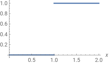
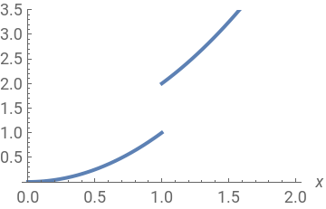
But the derivative of this function involves the impulse Dirac Delta distribution concentrated at , so indeed cannot be considered continuous there:
x=1
f'(x)
In[]:=
D[+HeavisideTheta[x-1],x]
2
x
Out[]=
2x+DiracDelta[-1+x]
3.1.2 Sin[x]/x
3.1.2 Sin[x]/x
As to the function , it illustrates the view point difference between math purists and engineers (I am in the latter camp). This function, or its extension , is continuous at zero for two reasons.
Sin[x]/x
Sinc[x]
First, because, again, its limit, its limit from the left, and its limit from the right are all equal to each other:
In[]:=
Limit,x->0,Limit,x->0,Direction->"FromAbove",Limit,x->0,Direction->"FromBelow"
Sin[x]
x
Sin[x]
x
Sin[x]
x
Out[]=
{1,1,1}
And second, is just a point of an apparent discontinuity, which clearly disappears upon Taylor expansion and the division of the respective series:
x=0
In[]:=
Series[Sin[x],{x,0,5}]xSeries,{x,0,5}
Sin[x]
x
Out[]=
x-++
3
x
6
5
x
120
6
O[x]
Out[]=
x
Out[]=
1-++
2
x
6
4
x
120
6
O[x]
In summary, the purists could see the difference between and , but engineers would not. Since I am big on viewpoint diversity, let’s agree to disagree 😀.
Sin[x]/x
Sinc[x]