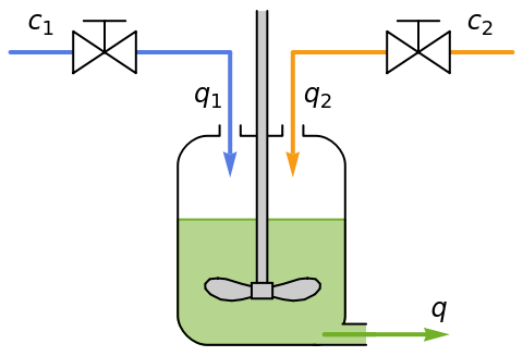
Improve the response of the flow rate in a mixing tank:
|
In[]:=
tank=StateSpaceModel,,DescriptorStateSpace->True,/.->+/.
q
0
q
10
q
20
Out[]=

| | | input flow rate 1 | input flow rate 2 | ||||
tank volume | 1 | 0 | 0 | 0 | 0 | -1 | 1 | 1 |
tank concentration | 16.6667 | 1000 | 0 | 0 | -30. | -16.6667 | 10. | 20. |
output flow rate | 0 | 0 | 0 | 0.015 | 0 | -1 | 0 | 0 |
output flow rate | | | | 0 | 0 | 1 | 0 | 0 |
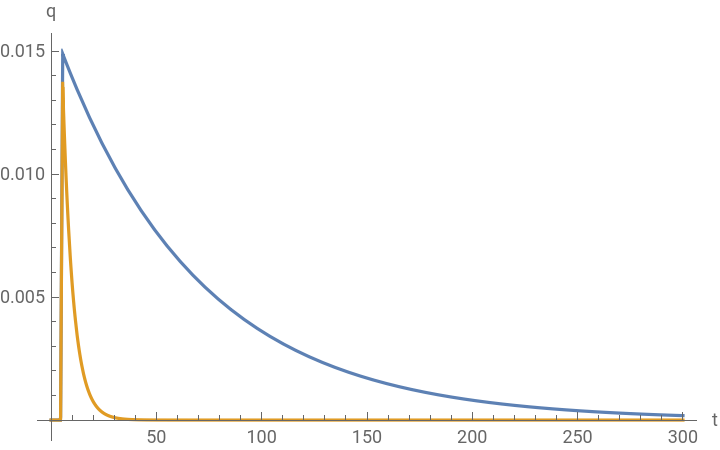
The response to a disturbance in the flow rate is sluggish:
q
2
In[]:=
or
ol
or
ol
Out[]=
Design a state-feedback controller to accelerate the response:
In[]:=
p={-0.2,-0.03};=StateFeedbackGains[tank,p,"Data"]
Out[]=
SystemsModelControllerData


The closed-loop system:
In[]:=
csys=["ClosedLoopSystem"]//Chop
Out[]=
| 1 | 0 | 0 | -0.185 | 0 | -1. | 1. | 1. |
| 16.6667 | 1000 | 0 | -3.08333 | -30. | -16.6667 | 10. | 20. |
| 0 | 0 | 0 | 0.015 | 0 | -1. | 0 | 0 |
output flow rate | | | | 0 | 0 | 1. | 0 | 0 |
The response of the closed-loop system is faster:
In[]:=
or
cl
or
ol
or
cl
Out[]=