Abstract: Every day, there are 93,000 global flights, carrying millions of passengers. Something that planes are quite unsuccessful in currently is flying the most efficient path between those locations, and frequently, in order to avoid lack of organization, many planes can't fly through their most efficient path. But how costly is this? And, with the outside factor of wind, is it possible to fly the most efficient flight path for any flight? I conducted a case study for a flight from Los Angeles to New York City in order to answer this question.
Introduction:
Introduction:
There were two cases of differing wind orientations: Case 1 was a simpler case, where wind blew at a constant velocity in a constant direction while Case 2 was far more complicated, with the wind direction changing en-route. For case 2, by iterating through different trajectories, I computed the fastest route, and collected data regarding total flight time, airplane direction, and airplane location during wind changes. This data was compiled into an image of the flight route that the plane would have to take. I concluded that a 3rd case would need to be done with a slightly different methodology to provide more insightful results. The beginning of my project entailed analyzing the shortest distance route and real world plane routes from Los Angeles to NYC (assuming no wind). Seeing the difference between the two scenarios will give us a measurement of how impactful this project would be.
In[]:=
EntityList[EntityClassList["Airport"]];
In[]:=
x=EntityList;y=RandomInteger[Length[x]];z=RandomInteger[Length[x]];shortened={Part[x,y],Part[x,z]}

Out[]=
,
Takes two completely random airports
In[]:=
coord1=Interpreter[Part[shortened,1]]["Coordinates"]coord2=Interpreter[Part[shortened,2]]["Coordinates"]GeoPosition[coord1]
Out[]=
{-5.66667,-43.535}
Out[]=
{37.6293,-77.7475}
Out[]=
GeoPosition[{-5.66667,-43.535}]
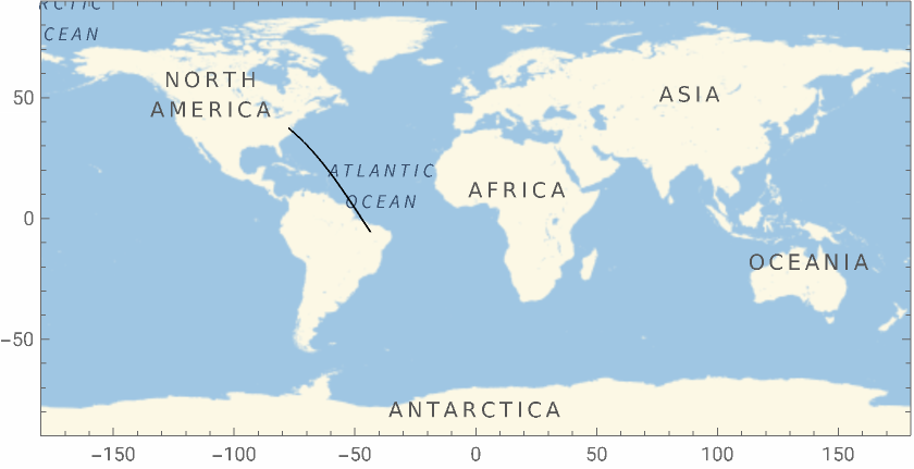
Returns the shortest distance distance between the 2 flights. The purpose of this was to verify how the GeoPath function worked with different locations.
In[]:=
GeoGraphics[GeoPath[{coord1,coord2}],GeoRange"World",FrameTrue]
Out[]=
Calculating optimal vs. real flight comparisons for flights from Los Angeles to New York City
Calculating optimal vs. real flight comparisons for flights from Los Angeles to New York City
This section will work primarily with comparing how flights behave right now to observe the impact of this project.
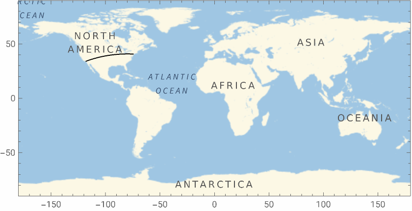
The shortest Distance a plane can fly LA to New York City and the distance it would travel
In[]:=
GeoGraphicsGeoPathInterpreter["Coordinates"],Interpreter["Coordinates"],GeoRange"World",FrameTrueGeoDistance,
Out[]=
Out[]=
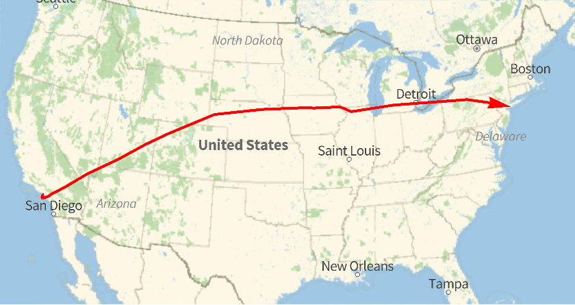
Returns a real life flight on a map from LA to NYC, as well as the distance it would entail.
In[]:=
realflight=FlightData,"FlightMap"
Out[]=
In[]:=
FlightData,"DistanceTraveled"
Out[]=
The images are very different, but this is because, in practice, planes cannot fly in one direct line to their destination, and air traffic forces planes to go through certain directions, hence the choppy, straight lines. In fact, hundreds of miles are added onto the trip because of this choppiness. These results imply that optimizing the direction of plane traffic with regards to their most efficient paths is an issue that could reduce a significant amount of fuel.
Case 1: Introduction
Case 1: Introduction
The past code assumes no wind, but the rest of this project will take wind direction into consideration and optimize the direction of the plane based on that data. I decided for there to be a velocity of 15.7m/s of headwind coming directly west (headwind). We assume that the velocity of the plane is 122 m/s, but this is variable on the airplane model. All other conditions are the exact same.
In order to accomplish getting the plane to its destination fastest, I needed to break both velocity vectors into their longitudinal and latitudinal components. The sum of the latitudinal vectors and longitudinal vectors will result in the actual direction of the plane. The result is this:
In order to accomplish getting the plane to its destination fastest, I needed to break both velocity vectors into their longitudinal and latitudinal components. The sum of the latitudinal vectors and longitudinal vectors will result in the actual direction of the plane. The result is this:
Thetaw (angle of the direction wind takes ) is 180 because the wind is going directly west. vertvelocity is the vertical velocity of the plane given the headwind from the plane. horizvelocity serves the same purpose but it is the horizontal component.
In[]:=
thetaw=180vertvelocity=Sin[thetawDegree]*15.7+Sin[thetapDegree]*122horizvelocity=Cos[thetaw]*15.7+Cos[thetap]*122
Out[]=
180
Out[]=
0.+122Sin[°thetap]
Out[]=
-9.39582+122Cos[thetap]
Note that thetap is the angle above the parallel to the equator that the plane is flying at, in other words the direction of the plane.
Case 1: Establishing equation variables
Case 1: Establishing equation variables
Because Los Angeles and New York are fixed points, using their coordinates we can detect how high up and how far east the plane actually went. This will be critical in solving for the flight time in air, and thetap.
In geometry, via the equation S= r (ϴ), you are able to extract arc length S given the radius of the circle, and the angle in radians separating the radii at the arc length endpoints.
In[]:=
latitudeheight=UnitConvert*QuantityMagnitudeLatitude-Latitude*Pi180,"Kilometers"
Out[]=
Computes the same variable but horizontally.
In[]:=
longitudeheight=UnitConvert*QuantityMagnitudeLongitude-Longitude*Pi180,"Kilometers"
Out[]=
Gives the angle above horizontal at which the plane would fly during its direct route.
In[]:=
ArcTan[latitudeheight/longitudeheight]/Degree
Out[]=
8.49804
Case 1: Solving Equation variables
Case 1: Solving Equation variables
Finally, all that’s left to do in this code is solve the different equations for time and thetap. This can be done with the solve function:
In[]:=
Solve[longitudeheight*1000/time==-15.7+Cos[thetapDegree]*250&&latitudeheight*1000/time==Sin[thetapDegree]*250,{thetap,time}]

Out[]=
thetap-170.97,time,thetap7.96631,time
Note: We multiply longitude height and latitude height by 1000 to convert from km to m. The equations say that the distance travelled divided by the time travelled is equivalent to the net velocity of the plane.
In[]:=
thetap-170.9702271886978`,time,thetap7.966312449803552`,time
Out[]=
thetap-170.97,time,thetap7.96631,time
Conclusions from Case 1:
Conclusions from Case 1:
Overall, our final data makes sense, because it does take longer for the plane to fly against these headwinds with the wind slowing the plane down, and thetap decreases, meaning that the plane points more east (7.96631 as opposed to 8.49804 ). This also makes sense, as we can consider the plane needing to “fight” the wind more. This is a relatively successful case.
Case 2: Introduction
Case 2: Introduction
Case 2 is far more complicated than case 1; there are two different wind speeds, one being 20 m/s at 45 Degrees Northwest and the other being 15 m/s at 330 Degrees (30 Degrees below the horizontal) Southwest. The plane experiences these winds at different times, as they are split by a line (called later in this project the partition line) where the winds switch direction. The partition line is 8.49804 Degrees askew east from being a perfectly vertical longitude line. Initially, all I do is define variables I will need.
What is most complicated is that there are not 2 clear cut points where the route needs to come from and go to: because the wind changes instantaneously, so will the direction of the plane. So, instead of solving for the new takeoff direction of the plane like in Case 1, I will use the table function to iterate the angle above the horizontal the plane will fly at from 1-90. Based on the trajectory of the plane, it will hit the partition line at different points. However, if one is able to calculate where this point is, you could apply the same logic used in Case 1 but treat the calculated point as the place the plane traveled from (in other words, the varied point is comparable to Los Angeles in Case 1). Calculating this point can be done graphically with Solving 2 systems of equations: one being the partition line and the other being the line of the plane’s trajectory.
The next part of the code is the defining of variables. The code stores variables to the data that will be used later. The first 2 variables are the coordinates of Los Angeles and its Airport.
This stores variables for the coordinates of NYC. These coordinates (a well as Los Angeles’s) will be used to detect where the plane starts and ends at.
The next two variables mark the origin of what I will turn into my linear, 2D graph. The graph’s objective is to find the solution to the system of equations of the lines created by the route of the plane and the partition line in order to show where the plane will be when the wind changes direction.
This line puts the coordinates of Los Angeles in the context of the 2D graph.
Finds the slope of the partition line (this gives us all we need to find the equation of the partition line, as it is a given in the way I established my graph that the partition line crosses the origin).
Initializes the best coordinates that the plane goes to on the partition line (based on time). While iterating, this value will only change if the plane going to this coordinate location will result in less flight time.
Initializes theta and time at 0. secondthetap is the angle below the horizontal at which the plane will fly after the partition line to fly to New York City.
The function fa gives us the actual angle of the plane given the defined wind conditions prior. In other words, planeangle is where the plane is pointing to, while fa gives us where the plane is actually going.
Now that we have the actual direction of the plane, we can calculate the direction of the plane in y=mx+b form, where findB solves for b. m is the tangent of the angle calculated in fa (slope of plane direction), and the coordinates of LAX are {x,y}.
solve1 is the first system of equations, and its significance is to find where the plane reaches the point where the winds change direction. {x, y } represents coordinates
getLegOneTime computes the time it took the plane to get to {locx, locy}
This next function helps us attain the second angle the plane will fly at after crossing the partition line (thetap):
The next code helps us attain the time the plane was in the flight post- partition line.
The next functions focus on the route from {locx, locy} to JFK. findVertDistance finds the vertical distance the plane travelled to get to New York.
This function accomplishes the exact same thing for horizontal distance.
Finally, we must solve for the time it takes to get from {locx. locy} to JFK. solve2 solves this given the same methodology used in Case 1 (as beginning point and end point are given). It also calculates the angle at which below the horizontal the plane will fly at.
Initializes the optimal time in flight and angle of flight above the horizontal to be the first case of the plane going at one degree.
Getting the Results:
Getting the Results:
Best time is initialized at a high number because it should be switched immediately to the time of the first iteration.
The table function iterates for 0 Degrees to 90 Degrees, with iraw being the given variable for the direction of the plane without wind. Firstly, we use solve1 to get the coordinates of the partition line the plane would get to. We then check if these coordinates are in the given range that latitude and longitude could be at, because otherwise it could run an error. If the coordinates are real coordinates, then I used the functions from above to calculate how much time the trip would take going through mysterycoords. If that time is the best time so far, we change our initialized variables: besttheta and bestloc to the more optimal solution. The loop returns a list of nulls and coordinate points, where the coordinate points are instances in the iteration were the table function found a better solution. The list of numbers are coordinates.
The table function iterates for 0 Degrees to 90 Degrees, with iraw being the given variable for the direction of the plane without wind. Firstly, we use solve1 to get the coordinates of the partition line the plane would get to. We then check if these coordinates are in the given range that latitude and longitude could be at, because otherwise it could run an error. If the coordinates are real coordinates, then I used the functions from above to calculate how much time the trip would take going through mysterycoords. If that time is the best time so far, we change our initialized variables: besttheta and bestloc to the more optimal solution. The loop returns a list of nulls and coordinate points, where the coordinate points are instances in the iteration were the table function found a better solution. The list of numbers are coordinates.
Note: this may take 3040 seconds to compile
This data gives us that a plane flying at 25 degrees should hit the partition line at coordinates {13.9781,-68.4259} and should take 104214 seconds (28.94 hours)
The image of the route the plane would travel
The endpoints of the line in the Atlantic Ocean are the other 2 points that were more optimal that the points before, and given this information it is clear why {13.9781,-68.4259} was considered the most optimal coordinate
Final Conclusions:
Final Conclusions:
I found Case 1 to be a relatively successful case, where the math seemed more secure and intuitive to the project. The results were relatively sensible, as the angle did tighten and the duration of the flight was also very similar to what we would expect with winds slowing us down.
As for case 2, the given graphic is not completely similar to the expected graphic because the plane goes significantly more south than what I would have expected. This error could be due to the fact that converting the route of the plane on a 2D graph distorted the route, and made our data inaccurate. Also, not having access to real data made my data slightly less realistic. Although I did not have time at the camp, due to how much I liked the project, I plan on adding a third case, where I take advantage of a lot more commands Wolfram uses, primarily the functions that are specifically used for our world (like the functions beginning with Geo). Geo functions will help me account for the curvature of the earth in a way that is significantly more accurate and simpler for myself.
As for case 2, the given graphic is not completely similar to the expected graphic because the plane goes significantly more south than what I would have expected. This error could be due to the fact that converting the route of the plane on a 2D graph distorted the route, and made our data inaccurate. Also, not having access to real data made my data slightly less realistic. Although I did not have time at the camp, due to how much I liked the project, I plan on adding a third case, where I take advantage of a lot more commands Wolfram uses, primarily the functions that are specifically used for our world (like the functions beginning with Geo). Geo functions will help me account for the curvature of the earth in a way that is significantly more accurate and simpler for myself.
More Aspects of the project to think about and future works:
More Aspects of the project to think about and future works:
Part of the project that was quite difficult, especially in the beginning, was to evaluate how to measure the impact wind would have on the airplane. What wind really is, is a series of many collisions that hit an aeroplane and slow it down by minimizing the magnitude of its momentum. However, after reading online, many people simply summed the vectors of wind and plane speed, and that was what I eventually did in my project. However, making a project on seeing how wind could be considered a change in momentum would be interesting to see.
Also, for this project I only analyzed a change of wind occurred only once en route. Running a test where wind changes, say, 100 times, would make iterating the angle 1 through 90 pretty inefficient and impractical. A Monte Carlo simulator could be used in these simulations to further develop this project and find more ways of making it realistic.
Finally, accessing and downloading real atmospheric wind data from the continental United States could be really interesting to implement, and although I couldn’t find it for my project, it would make the project significantly more relevant.
Acknowledgements
Acknowledgements
I would like to give a huge thanks to my mentor Athanasios, Karan, and Nora who helped me develop my code and find my interesting way of writing my code.
References
References
◼
Benson, Tom Benso. “Effect of Size on Drag.” NASA, www.grc.nasa.gov/www/k-12/VirtualAero/BottleRocket/airplane/sized.html. Accessed 12 July 2023.
◼
“Challenge 6 – as the Crow Flies on a Spherical Planet.” NASA, eclipse2017.nasa.gov/crow-flies-spherical-planet. Accessed 12 July 2023.
◼
R Nave. “Airplane in Wind.” Airplane in Wind, www.hyperphysics.phy-astr.gsu.edu/hbase/airpw.html. Accessed 12 July 2023.
◼
Zhu. “Flight Environment PREVAILING WINDS.” Prevailing Winds, www.weather.gov/source/zhu/ZHU_Training_Page/winds/Wx_Terms/Flight_Environment.htm#:~:text=These%20jet%20stream%20segments%20move,between%20100%20and%20150%20knots. Accessed 13 July 2023.
CITE THIS NOTEBOOK
CITE THIS NOTEBOOK
Finding optimized route for planes flying from Los Angeles to New York City
by Marco Giordano
Wolfram Community, STAFF PICKS, July 13, 2023
https://community.wolfram.com/groups/-/m/t/2963799
by Marco Giordano
Wolfram Community, STAFF PICKS, July 13, 2023
https://community.wolfram.com/groups/-/m/t/2963799