This project was part of a Data Science module, taught by Jozsef Konczer at Milestone Institute. For anyone interested in some materials here is a GITHUB.
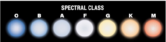
Stars are usually classified by their spectral characteristics under the Morgan-Keenan system. This classification can be quite accurately done by looking at the temperatures of the stars, but I was interested if I can train an AI classifier using other characteristics of stars.(The main spectral classes in the MK system)
Assembling the training set
Assembling the training set
Mathematica’s database conveniently includes data on more than 200 000 stars with many characteristics. Unfortunately most of these have a lot of missing information. We have to filter these out to get a dataset which we can use to train then test our classifier. This is going to be the hardest part of the project.
Even after we filtered the dataset we have to select the specific characteristics we want to compare. We will be looking at the stars’ mass, absolute magnitude and luminosity and classifying them to their spectral class. It is important to note that in the MK system the precise spectral classification is a three component expression: the first part is the spectral class (usually O - B - A - F - G - K - M), the second part is the spectral subclass (using numbers from 0 to 9), and the third part is a roman numeral depicting luminosity. This would be too specific for the classifier, so we will stick to the main spectral class.
In[]:=
StarData["Sun","SpectralClass"]
Out[]=
G2V
In[]:=
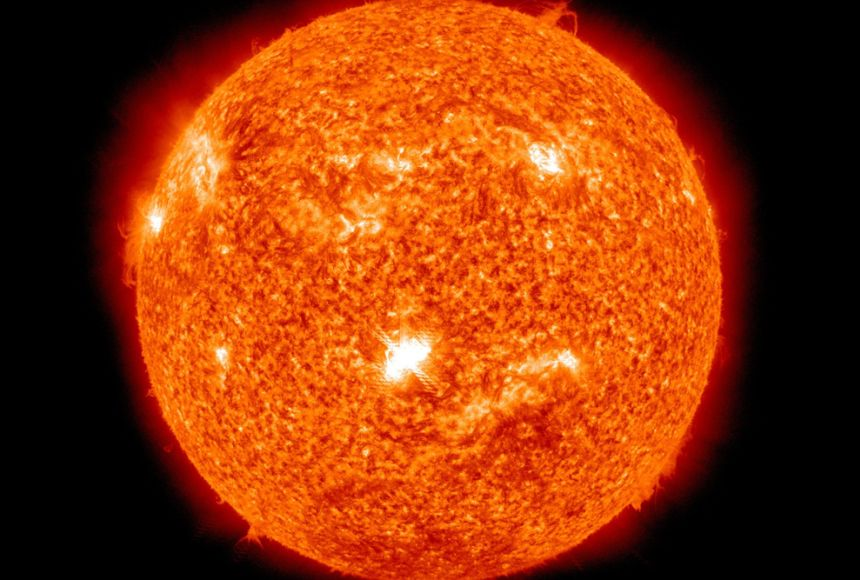
As we can see, the Sun’s specific spectral class is G2V, with the following code we will only look at it as a class G star.
In[]:=
Length[EntityList["Star"]]
Out[]=
213202
In this part we will filter out every star that has missing data for their mass, absolute magnitude and luminosity. For easier access, we also export this so that we do not have to run this code again. The main code is commented out but anyone is welcome to try it out for themselves.
(*ShallowdataEntity=EntityListFilteredEntityClass"Star",EntityFunctione,e["Mass"]>&&Exp[e["AbsoluteMagnitude"]]>0&&e["Luminosity"]>//AbsoluteTiming*)
Out[]=
80.1806,,,,,,,,,,,38729
(*Export[NotebookDirectory[]<>"StarEntityList.mx",dataEntity]*)
Shallow[dataEntity=Import[NotebookDirectory[]<>"StarEntityList.mx"]]
Out[]//Shallow=
,,,,,,,,,,38729
As we can see, we were able to reduce our dataset to about 38 000.
In[]:=
Length[dataEntity]
Out[]=
38739
Now this is the ‘big boy’ code of the project. Here, we will take our preliminary filtered list of stars and take the only details we need (name, mass, absolute magnitude, luminosity and spectral class) and create an association table from them. We export the final table into a .txt file (it is not a typical format, but we have not filtered the spectral class yet and there are missing data there that could cause some trouble; this way we eliminate the risk, better safe than sorry). The main code is commented out, I recommend not running the code itself because even on a beefier computer it would run for a day.
(*RunsforapproxaDay*)(*Monitor[rawData=Table[StarData[dataEntity[[k]],{"Name","Mass","AbsoluteMagnitude","Luminosity","SpectralClassList"},"PropertyAssociation"],{k,1,Length[dataEntity]}],{k,Length[dataEntity]}]Export[NotebookDirectory[]<>"FilteredRawData.txt",rawData]*)
Because of the .txt format, while importing we need to specify what type of expression we want Mathematica to import the data into.
In[]:=
dataFilteredRaw=ToExpression[Import[NotebookDirectory[]<>"FilteredRawData.txt","List"]];
In[]:=
Length[dataFilteredRaw]
Out[]=
38739
We got every star back after the property association code, yay!
Here we will set up two filtration rules. The first one is a redundant filter for the three characteristics (mass, absolute magnitude and luminosity), still better be safe than sorry. The second one filters out stars that have their main spectral class missing.
In[]:=
ruleDeleteMissing1=<|___,_->Missing[___],___|>:>Nothing[];ruleDeleteMissing2=<|___,"SpectralClassList"->{Missing[___],___},___|>:>Nothing[];
In[]:=
dataChecked=dataFilteredRaw/.{ruleDeleteMissing1,ruleDeleteMissing2};
In[]:=
Shallow[dataChecked]
Out[]//Shallow=
Name2MASS J0523-1403,Mass,AbsoluteMagnitude20.6,Luminosity,SpectralClassList{L,2.5,5},NameAcamar,Mass,AbsoluteMagnitude-0.591,Luminosity,SpectralClassList{A,4,3},NameAchernar,Mass,AbsoluteMagnitude-2.77,Luminosity,SpectralClassList{B,3,5},NameAchird,Mass,AbsoluteMagnitude4.59,Luminosity,SpectralClassList{G,0,5},NameAcrab,Mass,AbsoluteMagnitude-3.50,Luminosity,SpectralClassList{B,0.5,5},NameAcrux,Mass,AbsoluteMagnitude-4.23,Luminosity,SpectralClassList{B,0.5,4},NameAdhafera,Mass,AbsoluteMagnitude-1.08,Luminosity,SpectralClassList{F,0,3},NameAdhara,Mass,AbsoluteMagnitude-3.97,Luminosity,SpectralClassList{B,2,2},NameAin,Mass,AbsoluteMagnitude0.145,Luminosity,SpectralClassList{K,0,3},NameAlgedi,Mass,AbsoluteMagnitude0.966,Luminosity,SpectralClassList{G,Missing[Uncertain,{6,8}],3},38599
In[]:=
Length[dataChecked]
Out[]=
38609
We only had to discard around a hundred stars and now we have 38 609 stars that are ready for the classifier.
In[]:=
classCount=Tally[#["SpectralClassList"][[1]]&/@dataChecked]
Out[]=
{{L,1},{A,4888},{B,5212},{G,6172},{F,6986},{K,12911},{O,156},{M,2283}}
In[]:=
BarChart[Last/@classCount,ChartLabelsFirst/@classCount]
Out[]=
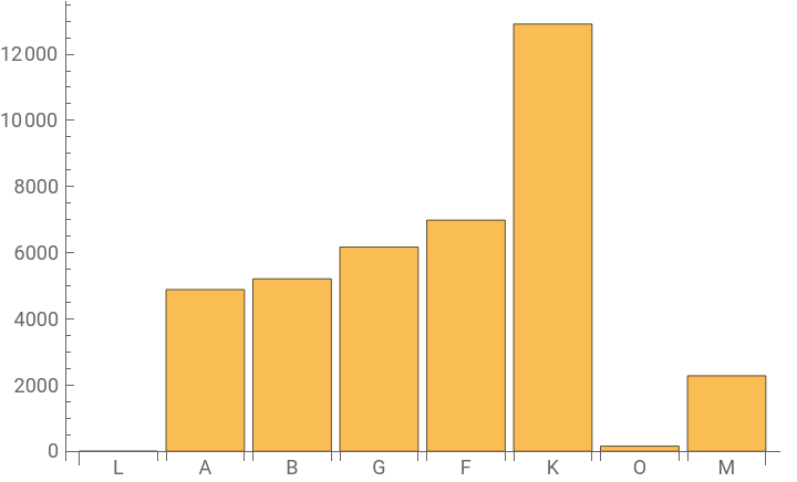
Looking at the chart we can see two things: first, the distribution of classes here are about close to the real world (only difference is that in our universe class M stars are the most common, the reason we have so few here is probably because they are very dim, so observing them is really hard); second: we have a single class L star...
While observing stars, scientists had to expand the Morgan-Keenan system with different classes (like D for white dwarfs or S and C for carbon stars, etc.), class L is one of these new classes introduced. These stellar objects are either brown dwarfs, supermassive gas giants that are just a bit too small to start hydrogen fusion; or incredibly dim red dwarfs that are barely large enough to facilitate nuclear fusion in their cores. We are lucky, if we look at the shallow list, our class L outlier is actually the first one on the list, it is the star ‘2MASS J0523-1403’. This star is located about 40 ly away from Earth and can be found in the constellation of Lepus. It is a low mass red dwarf star and currently is the smallest, dimmest and coolest star we know of, barely able to sustain hydrogen fusion. For the sake of our classifier we are going to remove it.
In[]:=
dataChecked7=DeleteCases[dataChecked,_?(#["SpectralClassList"][[1]]=="L"&)];
In[]:=
classCount7=Tally[#["SpectralClassList"][[1]]&/@dataChecked7]
Out[]=
{{A,4888},{B,5212},{G,6172},{F,6986},{K,12911},{O,156},{M,2283}}
We bid farewell to the L class star and now we only have the seven main classes (hence the ‘7’).
Here we will randomly select 80% of our stars to be the training set and let the rest be the test set. As their name suggest we will train the classifier with the training set and then try it out on the test set.
In[]:=
ratio=0.8;SeedRandom[1234];{training0,test0}=With[{RandomList=RandomSample[dataChecked7,Length[dataChecked7]]},{RandomList[[;;Floor[ratioLength[dataChecked7]]]],RandomList[[Floor[ratioLength[dataChecked7]]+1;;]]}];
In[]:=
Length[training0]Length[test0]
Out[]=
30886
We will create a table in which we associate the three characteristics to the spectral class so that our classifier knows what to do.
Training the classifier
Training the classifier
We are lucky, we only need one line of code (after all the prep work, of course) and Mathematica does the rest for us.
During training our classifier achieved a 87% accuracy. With how large numbers we are working with, this is incredibly good!
Build a test set
Build a test set
We do the same thing we did to our training set, we create a table where we associate the three characteristics with the spectral class.
Run the classifier
Run the classifier
Moment of truth: we are going to run our trained classifier on our prepared test set.
Evaluation
Evaluation
We can get the classifier’s accuracy and the confusion matrix pretty easily. We can see that we achieved a 84% accuracy, a beautiful result. If we look at the confusion matrix, we can see that the classifier had the most problem with M, K, G classes. The classifier was keen on predicting M and G stars as K stars, the explanation is simple: these three are the most common stars in the universe, as K is basically a middle ground it is easy to understand why it misclassified so many this way.
In the end we can be proud of our work, we were able to train a really accurate classifier. Obviously we are not going to revolutionise astronomy, but still a really great success.
CITE THIS NOTEBOOK
CITE THIS NOTEBOOK
Using basic attributes to predict stellar spectral classes
by Máté Kádas
Wolfram Community, STAFF PICKS, August 11, 2023
https://community.wolfram.com/groups/-/m/t/2988252
by Máté Kádas
Wolfram Community, STAFF PICKS, August 11, 2023
https://community.wolfram.com/groups/-/m/t/2988252