In[]:=
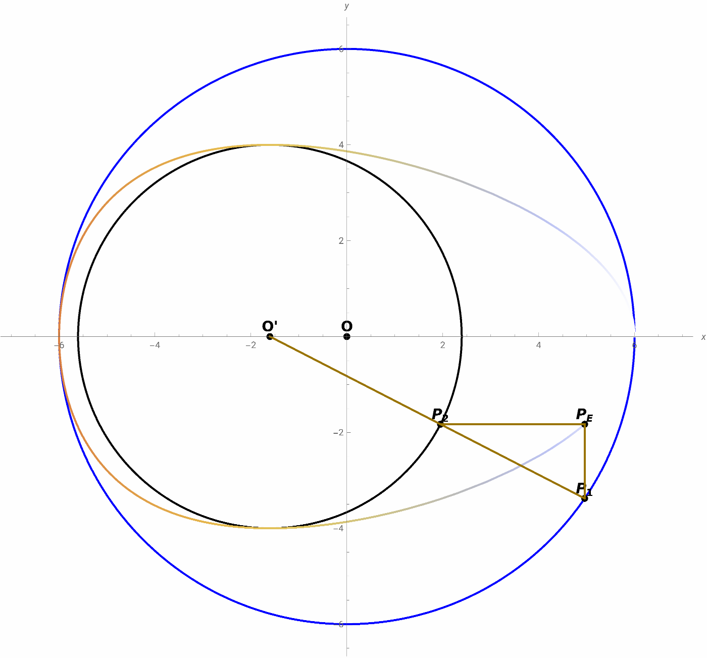
HügelschäfferEgg::usage="There are two circles, one with center at the origin and radius R, the other with center at (d, 0) and radius r. R > r, it is drawn a straight line from the center (d, 0) of the minor circle that forms an angle θ with the positive axis X. This line intersects the major circle in and the smallest in . The point (x, y) of the egg curve is obtaining by combining the x coordinate of the point and the y coordinate of the point . References: https://mathcurve.com; AI; Personal.";
P
1
P
2
P
E
P
1
P
2
Development:
Parametric equations:
ζ[t_]:={RCos[t],RSin[t]};[t_]:={rCos[t]+d,rSin[t]};ℒ:{d,0}+w(ζ[t]-{d,0});
ζ
min
In[]:=
{d+w(-d+RCos[t]),RwSin[t]};
Substituting in the equation (x - d) + y = :
2
2
2
r
Solve[+==,w];
2
(d+w(-d+RCos[t])-d)
2
(RwSin[t])
2
r
In[]:=
w--2dRdCos[t]++,w-2dRdCos[t]++;[t_]:=RCos[t],R-2dRCos[t]++Sin[t];
r
2
d
2
R
2
Cos[t]
2
R
2
Sin[t]
r
2
d
2
R
2
Cos[t]
2
R
2
Sin[t]
P
E
r
2
d
2
R
2
Cos[t]
2
R
2
Sin[t]
Cartesian Equation:
Eliminatex==RCos[t],y==R-2dRCos[t]++Sin[t],t//FullSimplify;
r
2
d
2
R
2
Cos[t]
2
R
2
Sin[t]
In[]:=
2
r
2
d
2
R
2
y
2
r
2
R
2
x
2
d
2
R
2
y
Animation:
In[]:=
ManipulateR=6;r=4;P2[t_]:=d+-2dRCos[t]++(-d+RCos[t]),R-2dRCos[t]++Sin[t];[t_]:=RCos[t],R-2dRCos[t]++Sin[t];ζ[t_]:={RCos[t],RSin[t]};[t_]:={rCos[t]+d,rSin[t]};O1={0,0};O2={d,0};Show[{ParametricPlot[ζ[θ],{θ,0,2π},PlotStyle->{Blue,Thick}],ParametricPlot[[θ],{θ,0,2π},PlotStyle->{Black,Thick}],ParametricPlot[[θ],{θ,0,t},ColorFunction->"BeachColors"],Graphics[{Black,PointSize[0.01],Point[O1],Text[Style["O",14,Bold],O1,{0,-1.2}],Point[O2],Text[Style["O'",14,Bold],O2,{0,-1.2}],Point[ζ[t]],Text[Style["",14,Bold],ζ[t],{0,-1.2}],Point[P2[t]],Text[Style["",14,Bold],P2[t],{0,-1.2}],Point[[t]],Text[Style["",14,Bold],[t],{0,-1.2}],Thick,{DarkYellow,Line[{O2,ζ[t]}],Line[{[t],P2[t]}],Line[{[t],ζ[t]}]}}]},AspectRatioAutomatic,AxesTrue,AxesOrigin{0,0},AxesLabel{x,y},PlotRange{{-6.5,6.5},{-6,6}},ImageSize700],Style["Hügelschäffer Egg",Bold,Large],{{t,0.00002,"Value (t)"},0.000001,2π,0.00001},Delimiter,{{d,-1.60421,"Value (d)"},-2,2,0.00001},ControlPlacementTop
r
2
d
2
R
2
Cos[t]
2
R
2
Sin[t]
r
2
d
2
R
2
Cos[t]
2
R
2
Sin[t]
P
E
r
2
d
2
R
2
Cos[t]
2
R
2
Sin[t]
ζ
min
ζ
min
P
E
P
1
P
2
P
E
P
E
P
E
P
E
P
E
Out[]=


In 3D:
In[]:=
ManipulateR=6;r=4;d=-1.60421;ShowRevolutionPlot3DRCos[t],R-2dRCos[t]++Sin[t],0,{t,0,2π},{θ,0,θ1},RevolutionAxis{1,0,0},PlotStyle->Opacity[0.8],MeshFalse,BoundaryStyleDirective[Black,Thick],PerformanceGoal"Quality",ColorFunction"BeachColors",ParametricPlot3D[t{1,0,0},{t,-7,7},PlotStyle->{DarkGreen,Thick}],Graphics3D[{Black,Ball[{d,0,0},0.15],Ball[{d,rCos[θ1],rSin[θ1]},0.15],Dashed,Thick,Line[{{d,0,0},{d,rCos[θ1],rSin[θ1]}}]}],AxesLabel->(Style[#,15,Blue]&/@{"X","Y","Z"}),AxesOrigin{0,0,0},AxesTrue,BoxedFalse,BoxRatiosAutomatic,PlotRange7,ViewPoint{1.3,-2.4,2.},ImageSize700,Style["Hügelschäffer egg:",Bold,Large],{{θ1,0.00002,"Value (θ)"},0.00001,2π,0.00001},ControlPlacementTop
r
2
d
2
R
2
Cos[t]
2
R
2
Sin[t]
Out[]=

Verification:
Parametric equations { f[t], g[t] Cos[θ], g[t] Sin[θ] } :
When it rotates around X, the curve in XY plane { f[t], g[t], 0 } the coordinate y is multiplied by Cos[θ] and in the coordinate Z it is put coordinate y multiplied by Sin[θ], and it turns out:
Verification: