Summary of findings
Summary of findings
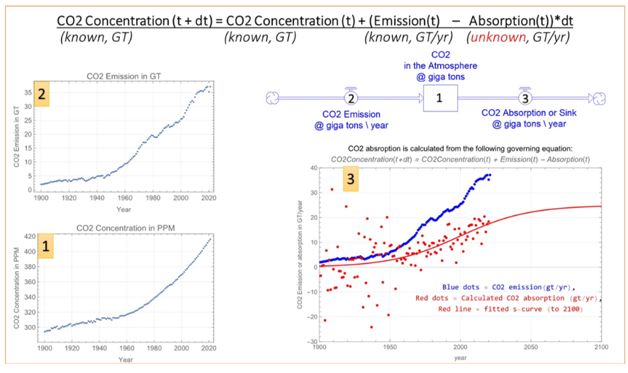
We calculated how much CO2 has been absorbed by the Earth using CO2 emission and concentration data. Our findings indicate that the Earth’s CO2 absorption has been increasing. We fitted an S-curve for CO2 absorption and it shows that the maximum capacity the Earth could absorb is 25 gigatons per year by 2050 (assuming the fitted S-curve represents the Earth’s climate accurately)
◼
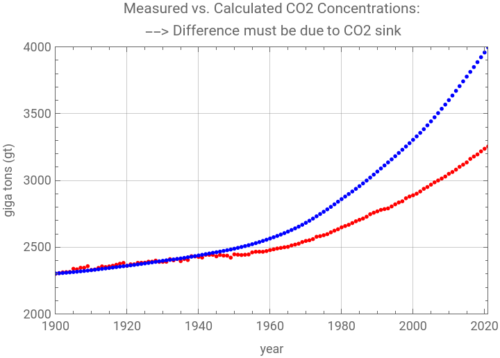
Hypothesis: If we initially ignore CO2 absorption or sink, then the accumulation of observed CO2 emissions should be equal to the observed CO2 concentration, as dictated by the governing equation. However, the accumulated CO2 emissions (i.e., CO2 concentration) are not equal to the CO2 concentration itself. Thus, it is logical to conclude that the difference between them is attributable to CO2 absorption.
Governing equation
Governing equation
◼
CO2 concentration (t+1) = CO2 concentration (t) + CO2 emission(t) - CO2 absorption(t), t = {1900,2021}, which is equal to the following equation
◼
∂Concentration(t)
∂t
◼
Data for CO2 concentration and CO2 emission are known and available, whereas the CO2 absorption or sink is unknown. Consequently, CO2 absorption can be computed using this governing equation.”
◼
Therefore, CO2 absorption(t) = CO2 concentration (t) + CO2 emission(t) - CO2 concentration (t+1)
◼
The fitted s-curve is
24.9108
1+
-0.041352(-1999.63+t)
Data source and terminology: CO2 emission and concentration data since “1900”
Data source and terminology: CO2 emission and concentration data since “1900”
◼
file name is “annual-co2-emissions-per-country.csv”
◼
CO2 emission in giga tons per year (Gt/yr).
◼
Primary factors are burning fossil oil (e.g., car) and land-usage (e.g., agriculture)
◼
◼
file name is “climate-change.csv” .
◼
CO2 absorption in giga tons per year == CO2 sink (Gt/yr).
◼
Primary factors are sink into sea and land-usage
◼
CO2 concentration in giga tons (Gt) == CO2 in the atmosphere == atmospheric CO2
◼
CO2 concentration is measured in PPM and converted to Gt by a factor of 7.82 (reference ?)
◼
The CO2 concentration data for several years between 1900 and 1953 are missing, and linear interpolation is applied.
Plots of CO2 emission and concentration
Plots of CO2 emission and concentration
In[]:=
(*Import["D:co2 data all sdlee v1.csv","CSV"]*)co2DataAll=;
In[]:=
co2EmissionGT=co2DataAll[[2;;,{1,2}]];co2EmissionPPM=co2DataAll[[2;;,{1,3}]];
In[]:=
co2ConcentrationPPM=co2DataAll[[2;;,{1,4}]];co2ConcentrationGT=co2DataAll[[2;;,{1,5}]];
In[]:=
(*CO2emissionandCO2concentration*)ListPlot{co2EmissionGT},,ListPlot{co2ConcentrationPPM},
Out[]=
,
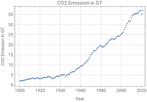
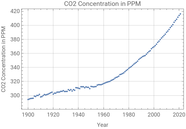
In[]:=
(*accumulationofCO2emission=calculatedCO2concentration*)calculatedCO2ConcentrationGT=Accumulate[co2EmissionGT[[All,2]]]+co2ConcentrationGT[[1,2]];years=co2DataAll[[2;;,1]];
◼
Accumulation of CO2 = calculated CO2 concentration
In[]:=
ListPlot[{co2ConcentrationGT,Transpose[{years,calculatedCO2ConcentrationGT}]},PlotLabel->"Measured vs. Calculated CO2 Concentrations:\n --> Difference must be due to CO2 sink",PlotStyle->{Red,Blue},PlotLegends->{"Red: Measured CO2 concentration (gt)","Blue: Calculated CO2 concentration =\n Accumulate[Measured CO2 emission] +\n CO2 concentration in 1900."},PlotRange->{{1900,2021},{2000,4000}},Frame->True,GridLines->Automatic,FrameLabel->{"year","giga tons (gt)"}]
Out[]=


◼
The difference between measured and calculated CO2 concentration must be due to CO2 sink.
In[]:=
co2ConcentrationGTTplus1=Transpose[{years,Append[Delete[co2ConcentrationGT[[All,2]],1],0.0]}];
◼
Calculate the CO2 absorption (main results)
In[]:=
(*co2absorption*)calculatedCO2AbsorptionGT=co2ConcentrationGT[[All,2]]-co2ConcentrationGTTplus1[[All,2]]+co2EmissionGT[[All,2]];(*thedatafor2021cannotbecomputedandthusdeleted*)calculatedCO2AbsorptionGT=Delete[Transpose[{years,calculatedCO2AbsorptionGT}],-1];
In[]:=
ListPlot[{co2EmissionGT,calculatedCO2AbsorptionGT},PlotRange->All]
Out[]=
Fit a s-curve
Fit a s-curve
◼
Assuming the fitted S-curve accurately represents Earth’s climate, the maximum absorption is about 25 gigatons per year, with approximately 5 GT remaining to reach maximum capacity. The year 2000 marked the midpoint of reflection.
In[]:=
co2AbsorptionNlmf1=NonlinearModelFit[calculatedCO2AbsorptionGT,maxL/(1+Exp[-k*(t-y0)]),{{maxL,25},{k,0.01},{y0,2000}},t];co2AbsorptionNlmf1//Normal
Out[]=
24.9108
1+
-0.041352(-1999.63+t)
In[]:=
Show[Plot[co2AbsorptionNlmf1[t],{t,1900,2100},PlotLabel->"CO2 absroption is calculated from the following governing equation:\nCO2Concentration(t+dt) = CO2Concentration(t) + Emission(t) - Absorption(t)",PlotLegends->Placed["Blue dots = CO2 emission(gt/yr), \nRed dots = Calculated CO2 absorption (gt/yr), \nRed line = fitted s-curve (to 2100)",{0.68,0.25}],PlotRange->{{1900,2100},{-30,40}},PlotStyle->{Red},ImageSize->500,Frame->True,FrameLabel->"year","CO2 Emission or absorption in GT/year",GridLines->Automatic],ListPlot[{co2EmissionGT,calculatedCO2AbsorptionGT},PlotStyle->{Blue,Red}]]
◼
References
◼
Ballantyne, A., Alden, C., Miller, J. et al. Increase in observed net carbon dioxide uptake by land and oceans during the past 50 years. Nature 488, 70–72 (2012). https://doi.org/10.1038/nature11299
CITE THIS NOTEBOOK
CITE THIS NOTEBOOK
Calculation of CO2 sink or absorption
by Sangdon Lee
Wolfram Community, STAFF PICKS, May 30 2023
https://community.wolfram.com/groups/-/m/t/2927367
by Sangdon Lee
Wolfram Community, STAFF PICKS, May 30 2023
https://community.wolfram.com/groups/-/m/t/2927367