Wolfram Cloud Document

ORIGINAL ARTICLE: Justin C. Feng, Shinji Mukohyama, and Sante Carloni (2024), Singularity at the demise of a black hole, Phys. Rev. D 109, 024040. https://doi.org/10.1103/PhysRevD.109.024040
arXiv Page

Article Abstract: We consider a class of quasiregular singularities characterized by points possessing two future-directed light cones and two past-directed light cones. Such singularities appear in the

1+1

trousers spacetime and the Deutsch-Politzer spacetime. We argue that these singularities are relevant for describing the end point of an evaporating black hole and show that a class of emergent Lorentz signature theories can provide a microscopic description for these singularities.

This notebook was written in Mathematica 13.3.1.0, using the tensor algebra suite

xAct

(v. 1.2.0)

Motivation

Introduction

This work concerns the conformal diagram for a 1+1 evaporating black hole in a “baby universe” scenario, in which spacetime extends beyond the black hole singularity. The termination of the event horizon in this case is in fact a kind of quasiregular singularity, characterized by points possessing two future-directed light cones and two past-directed light cones. Such singularities appear in the 1+1 trousers spacetime; the 1+1 evaporating black hole is in fact conformal to a region of the latter.

This Mathematica file contains calculations describing these singularities in terms of emergent Lorentz signature theories.

Black hole evaporation

Black hole conformal diagrams

Conformal diagrams (also known as Penrose diagrams) are useful for depicting the global causal structure of spacetime [Hawking and Ellis, The Large Scale Structure of Space-Time (Cambridge Univ. Press, 1973)].When constructing a conformal diagram, a spacetime of infinite extent is conformally mapped into a diagram of finite size. The conformal mapping preserves angles, so that null directions (and consequently causal relations) are preserved.

Evaporating d+1 black hole

Below is a conformal diagram of an evaporating asymptotically flat spherically symmetric black hole:

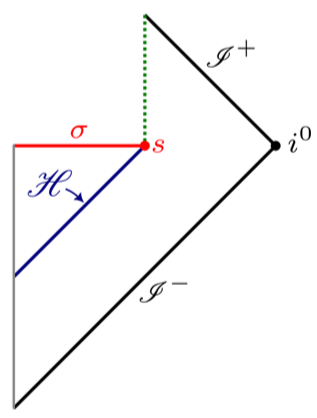
Points in the diagram represent

dimensional spheres, and

45°

lines correspond to radial null geodesics (light rays). The point

denotes spatial infinity,

denotes future null infinity (where outgoing light rays terminate), and

denotes past null infinity (where ingoing light rays originate). The surface

denotes the event horizon,

denotes a Schwarzschild-like singularity, and

is the endpoint of the black hole. The vertical lines correspond to limit points where the

dimensional spheres have zero “areal” radius.

Evaporating 1+1 black hole

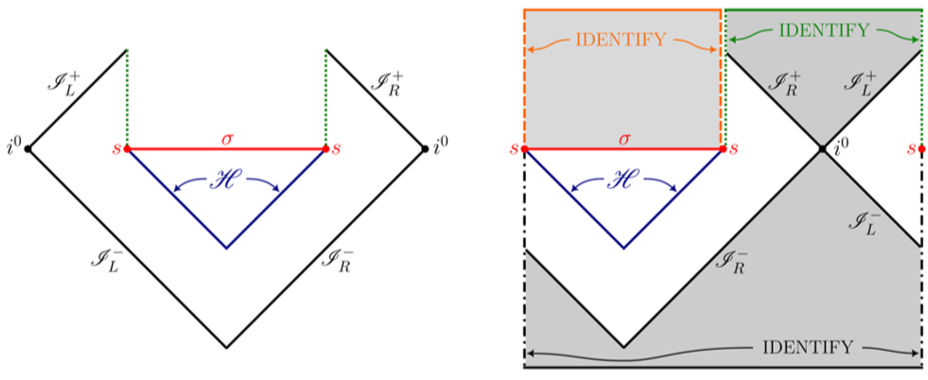
Conformal diagram for a

1+1

evaporating black hole:

Again,

45°

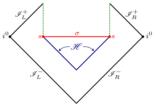
lines correspond to radial null geodesics (light rays), but in the

1+1

case, points genuinely represent points. In this case, future null infinity is split into two surfaces

and

and past null infinity is likewise split into two surfaces

and

Saddlelike quasiregular singularities and the trousers spacetime

A key question concerns the nature of the point

, where the horizon terminates. Here, it will be argued that

is closely related to a quasiregular singularity.For more on quasiregular singularities, see [Ellis and Schmidt, Gen. Relativ. Gravit. 8, 915–953 (1977)].

Saddlelike quasiregular singularities

Lorentzian spacetime manifolds have the property that each point has one future light cone and one past light cone. A saddlelike quasiregular singularity is one characterized by points with two future light cones, and two past light cones. Such a singularity can be constructed with a cut and past procedure in flat spacetime. This is illustrated below:

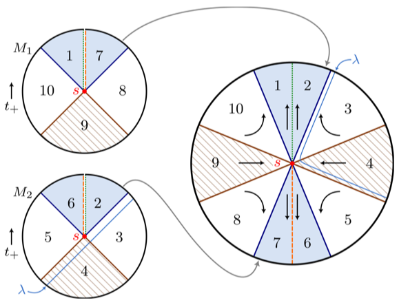
The two disks on the left,

and

, are two regions of Minkowski space (

45°

lines corresponding to null geodesics). The time direction is vertical, with time increasing upwards. The solid shaded regions are future light cones of the point

, and the hatched regions are past light cones. One can construct a saddlelike quasiregular singularity by cutting along the vertical dotted lines, and gluing so that region

is glued to region

, and region

is glued to region

.The result of the gluing is illustrated to the right. The diagram on the right is deformed so that

45°

lines are not null; note that the blue line

is bent on the right. The black arrows indicate the direction of positive time---the qualitative behavior resembles that of a saddle point of a dynamical system.

Trousers spacetime

One example of a quasiregular singularity is that of the

1+1

trousers spacetime, which one can also construct via a cut and paste procedure from a region of flat

1+1

Minkowski spacetime [Anderson and DeWitt, Found. Phys. 16, 91–105 (1986)]. The procedure is illustrated below:

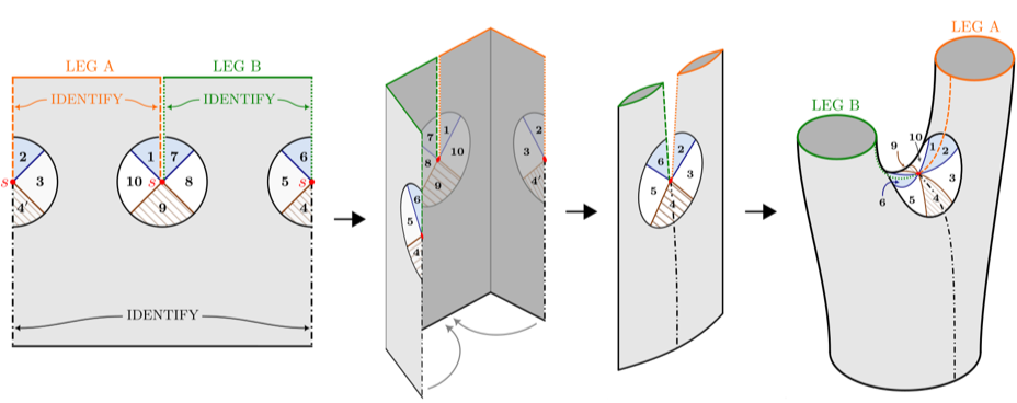
The diagram on the far left is a square region of 1+1 Minkowski spacetime (time is oriented vertically with

45°

lines corresponding to null geodesics). The diagram on the far right is a deformation to illustrate the topological equivalence to a pair of trousers.The point

is a saddlelike quasiregular singularity, and for obvious reasons, it is referred to in the literature as the crotch singularity.

the 1 + 1 evaporating black hole and the trousers spacetime

The 1+1 evaporating black hole is conformal to the flat 1+1 trousers spacetime; one can see this explicitly by pasting the conformal diagram directly onto the trousers spacetime:

Emergent Lorentz signature theories (tensor computations)

xAct Initialization

Summary

Load Packages

In[]:=

<<xAct`xTras`

Global

Settings

Definitions

Tensor Definitions

Here are the definitions for the constants and tensors used in the notebook.

Constants

Emergent Lorentz signature theory

General Overview

The basic idea is to consider a metric of the form:

Shift-symmetric euclidean quadratic scalar tensor theory

Einstein field equations (euclidean signature)

where:

Lagrangian

RULES

TERMS

“KINETIC” TERM

CURVATURE SQUARED TERMS

CURVATURE-GRADIENT INTERACTION TERMS

FOURTH-ORDER GRADIENT TERMS

FULL LAGRANGIAN

Field Equations

FIELD EQUATIONS - RAW

SCALAR EQUATION

METRIC EQUATION

Simplified field equations - scalar equation current form

CURRENT

VALIDATION

Simplified field equations - metric equation

SECOND-ORDER PART

METRIC PART

PURE CURVATURE PART

PURE SCALAR PART

MIXED PART

COMPARISON

TRACE OF FIELD EQUATIONS

Field Equations - Simplified Cases

FLAT, HARMONIC SCALAR PROFILE

SCALAR EQUATION

Ricci flat and Harmonic condition:

Condition for exact solution:

METRIC EQUATION

Zero-curvature and Harmonic condition:

Condition for exact solution:

Properties of Regularized Saddlelike Singularities

Clear xAct stuff:

Functions

1+1 Effective Geometry for a Regularized Quasiregular Singularity

Initialization

Metric Construction & Assumptions

Construction

Inverse & Connection

Inverse metric and connection are computed here.

Check that the connection coefficients vanish:

Curvature

Lowered Index Expressions

EVALUATION

DISPLAY

Check that the curvature is zero:

Scalar Field Profile

Scalar Field

CONSTRUCTION

Saddlelike profile:

GRADIENT

SECOND DERIVATIVE

TRACE OF SECOND DERIVATIVE

BACKGROUND GRADIENT NORM

Contour Plots

PLOT VARIABLES

SCALAR FIELD PLOT

Plot the level surfaces of the scalar field:

BACKGROUND NORM PLOT

Note that the level surfaces of the norm are circular.

Effective Metric

The effective metric is as follows:

Rules

Construction

MAIN

The inverse of the effective metric:

COUPLING REPLACEMENTS

Ricci Curvature

2D CASE

4D CASE

Determinant and Degenerate Surface

CONSTRUCTION

Determinant of the effective metric:

DEGENERATE SURFACE CONDITION

Tangent Vector

PARAMETERIZED SURFACE

PROJECTION OPERATOR

Projection operator:

NORM TANGENT

CITE THIS NOTEBOOK

Singularity at the demise of a black hole
by Justin C. Feng and Shinji Mukohyama and Sante Carloni
Wolfram Community, STAFF PICKS, February 15, 2024
https://community.wolfram.com/groups/-/m/t/3123688