The Optimum Equivalence Ratio at Various Gasification Temperatures
Housam Binous and Ahmed Bellagi
The Optimum Equivalence Ratio at Various Gasification Temperatures
Housam Binous and Ahmed Bellagi
Housam Binous and Ahmed Bellagi
We compute the optimum Equivalence Ratio (ER) of biomass gasification process based on thermodynamic equilibrium model. This
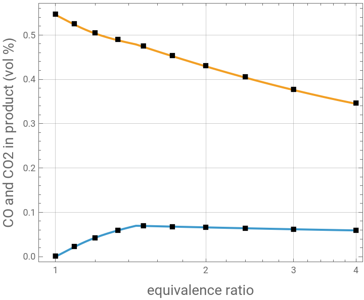
point is determined from the cross over point between CO2 and CO curves versus ER. Our results agree perfectly with their counterparts obtained using Aspen-Plus at T = 800K, 1000K and 1500K. This problem was presented in Ref. 1.
Reference:
[1] W. Jangsawang, K. Laohalidanond and S. Kerdsuwan, Optimum Equivalence Ratio of Biomass Gasification Process Based on Thermodynamic Equilibrium Model, Energy Procedia, Volume 79, 2015, pp. 520-527, https://doi.org/10.1016/j.egypro.2015.11.528
Cellulose: C6H10O5
Labels for number of moles:
n1 CH4
n2 H2
n3 H2O
n4 CO
n5 CO2
n6 NO
n7 NO2
n8 N2
n9 O2
n10 solid phase C
Cellulose: C6H10O5
Labels for number of moles:
n1 CH4
n2 H2
n3 H2O
n4 CO
n5 CO2
n6 NO
n7 NO2
n8 N2
n9 O2
n10 solid phase C
Labels for number of moles:
n1 CH4
n2 H2
n3 H2O
n4 CO
n5 CO2
n6 NO
n7 NO2
n8 N2
n9 O2
n10 solid phase C
In[]:=
P=1;
In[]:=
T=.
In[]:=
sol[x_,ER_]:=Quiet@FindMinimum[{Re[Gtot[x,P]],{n[7]<1/1000000,n[1]>0,n[2]>0,n[3]>0,n[4]>0,n[5]>0,n[6]>0,n[7]>0,n[8]>0,n[9]>0,n[10]>0},n[1]+n[5]+n[4]+n[10]6,4n[1]+2n[2]+2n[3]10,n[3]+n[4]+2n[5]+n[6]+2n[7]+2n[9]5+2×6ER,n[6]+n[7]+2n[8]2×0},Table[{n[j],0.01},{j,1,10}],MaxIterations10000,AccuracyGoal5];(*C6H10O5*)
Testing our code: set ER=1 and let us check that a complete combustion will occur (only CO2 and H2O will be present with CO2=6 moles and H2O=5 moles).
In[]:=
sol[1000,1][[2]]
Out[]=
{n[1]3.8713×,n[2]1.2391×,n[3]5.,n[4]9.76725×,n[5]6.,n[6]3.11338×,n[7]9.17445×,n[8]-2.01541×,n[9]1.12518×,n[10]1.19965×}
-9
10
-6
10
-7
10
-9
10
-10
10
-9
10
-6
10
-8
10
Testing our code : set ER = 1.2 > 1 and let us check that a complete combustion will occur (only CO2 and H2O will be present with CO2 = 6 moles and H2O = 5 moles) . Note that 1.2 moles of O2 will subsist.
In[]:=
sol[1000,1.2][[2]]
Out[]=
{n[1]-9.97021×,n[2]8.57529×,n[3]5.,n[4]8.37405×,n[5]6.,n[6]3.40288×,n[7]2.45668×,n[8]-2.92978×,n[9]1.2,n[10]5.39568×}
-10
10
-8
10
-8
10
-9
10
-9
10
-9
10
-9
10
T = 800 K
In[]:=
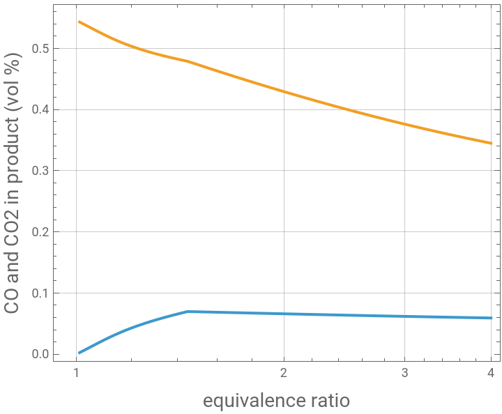
t1=Table[{1/ER,y[4]/.sol[800,ER][[2]]},{ER,0.25,1,0.02}]
Out[]=
{{4.,0.0591292},{3.7037,0.059791},{3.44828,0.0604291},{3.22581,0.061045},{3.0303,0.0616397},{2.85714,0.0622143},{2.7027,0.0627698},{2.5641,0.0633072},{2.43902,0.0638273},{2.32558,0.064331},{2.22222,0.064819},{2.12766,0.0652921},{2.04082,0.0657508},{1.96078,0.066196},{1.88679,0.066628},{1.81818,0.0670477},{1.75439,0.0674553},{1.69492,0.0678516},{1.63934,0.0682369},{1.5873,0.0686116},{1.53846,0.0689763},{1.49254,0.0693312},{1.44928,0.0695995},{1.40845,0.0662324},{1.36986,0.0627243},{1.33333,0.059128},{1.2987,0.0554155},{1.26582,0.0515556},{1.23457,0.0475143},{1.20482,0.0432567},{1.17647,0.0387511},{1.14943,0.0339778},{1.1236,0.028942},{1.0989,0.0236875},{1.07527,0.0183023},{1.05263,0.0129031},{1.03093,0.00760329},{1.0101,0.00248187}}
In[]:=
t2=Table[{1/ER,y[5]/.sol[800,ER][[2]]},{ER,0.25,1,0.02}]
Out[]=
{{4.,0.344828},{3.7037,0.352589},{3.44828,0.360156},{3.22581,0.367535},{3.0303,0.37473},{2.85714,0.38175},{2.7027,0.388598},{2.5641,0.39528},{2.43902,0.401802},{2.32558,0.408168},{2.22222,0.414384},{2.12766,0.420455},{2.04082,0.426384},{1.96078,0.432177},{1.88679,0.437837},{1.81818,0.44337},{1.75439,0.448778},{1.69492,0.454066},{1.63934,0.459237},{1.5873,0.464296},{1.53846,0.469245},{1.49254,0.474087},{1.44928,0.478792},{1.40845,0.481836},{1.36986,0.484934},{1.33333,0.488149},{1.2987,0.491511},{1.26582,0.495052},{1.23457,0.49881},{1.20482,0.502823},{1.17647,0.507124},{1.14943,0.511737},{1.1236,0.516656},{1.0989,0.521834},{1.07527,0.527177},{1.05263,0.532558},{1.03093,0.537852},{1.0101,0.542973}}
In[]:=
p1=ListLogLinearPlot[{t1,t2},PlotRange->All,Frame->True,AspectRatio->0.8,GridLines->Automatic,Joined->True,FrameLabel->{Style["equivalence ratio",14],Style["CO and CO2 in product (vol %)",14]}]
Out[]=
data obtained from Aspen - Plus simulation for benchmarking purposes
In[]:=
dataASPEN={{0.5,0.0517885588,0.272378273},{1,0.055331837,0.310924531},{1.5,0.0583296557,0.34552831},{2,0.0608993553,0.37664326},{2.5,0.0631267667,0.404698786},{3,0.0650761551,0.430079341},{3.5,0.0667966108,0.453120453},{4,0.0683262882,0.474111476},{4.5,0.0582748965,0.488975115},{5,0.0417602125,0.504267868},{5.5,0.0213938548,0.524108792},{6,2.6836092210^-10,0.545454545}};
In[]:=
t1a=Table[{6/dataASPEN[[i]][[1]],dataASPEN[[i]][[2]]},{i,1,Length@dataASPEN}];
In[]:=
t2a=Table[{6/dataASPEN[[i]][[1]],dataASPEN[[i]][[3]]},{i,1,Length@dataASPEN}];
In[]:=
p2=ListLogLinearPlot[{t1a,t2a},PlotRange->All,Frame->True,AspectRatio->0.8,GridLines->Automatic,PlotMarkers->Style["■",Black,12],FrameLabel->{Style["equivalence ratio",14],Style["CO and CO2 in product (vol %)",14]}]
Out[]=
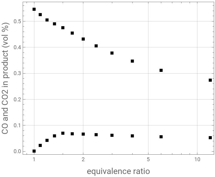
Aspen - Plus simulation vs. Mathematica code. We find perfect agreement
In[]:=
Show[p1,p2]
Out[]=
T = 1000 K
In[]:=
t1=Table[{1/ER,y[4]/.sol[1000,ER][[2]]},{ER,0.25,1,0.02}]
Out[]=
{{4.,0.424778},{3.7037,0.412963},{3.44828,0.401064},{3.22581,0.389107},{3.0303,0.37711},{2.85714,0.365091},{2.7027,0.353062},{2.5641,0.341036},{2.43902,0.329021},{2.32558,0.317027},{2.22222,0.305061},{2.12766,0.293129},{2.04082,0.281236},{1.96078,0.269388},{1.88679,0.257588},{1.81818,0.245841},{1.75439,0.234149},{1.69492,0.222517},{1.63934,0.210947},{1.5873,0.19944},{1.53846,0.188001},{1.49254,0.176629},{1.44928,0.165328},{1.40845,0.1541},{1.36986,0.142944},{1.33333,0.131864},{1.2987,0.120859},{1.26582,0.109931},{1.23457,0.0990815},{1.20482,0.0883104},{1.17647,0.0776186},{1.14943,0.0670067},{1.1236,0.0564751},{1.0989,0.0460243},{1.07527,0.0356545},{1.05263,0.0253661},{1.03093,0.0151587},{1.0101,0.00503258}}
In[]:=
t2=Table[{1/ER,y[5]/.sol[1000,ER][[2]]},{ER,0.25,1,0.02}]
Out[]=
{{4.,0.12166},{3.7037,0.133312},{3.44828,0.145075},{3.22581,0.15692},{3.0303,0.168822},{2.85714,0.180763},{2.7027,0.192726},{2.5641,0.204697},{2.43902,0.216665},{2.32558,0.22862},{2.22222,0.240553},{2.12766,0.252457},{2.04082,0.264327},{1.96078,0.276155},{1.88679,0.287939},{1.81818,0.299672},{1.75439,0.311352},{1.69492,0.322975},{1.63934,0.334538},{1.5873,0.346038},{1.53846,0.357472},{1.49254,0.368839},{1.44928,0.380137},{1.40845,0.391363},{1.36986,0.402516},{1.33333,0.413595},{1.2987,0.424598},{1.26582,0.435525},{1.23457,0.446374},{1.20482,0.457145},{1.17647,0.467836},{1.14943,0.478448},{1.1236,0.48898},{1.0989,0.49943},{1.07527,0.5098},{1.05263,0.520088},{1.03093,0.530296},{1.0101,0.540422}}
In[]:=
p1=ListLogLinearPlot[{t1,t2},PlotRange->All,Frame->True,AspectRatio->0.8,GridLines->Automatic,Joined->True,FrameLabel->{Style["equivalence ratio",14],Style["CO and CO2 in product (vol %)",14]}]
data obtained from Aspen - Plus simulation for benchmarking purposes
Aspen - Plus simulation vs. Mathematica code. We find perfect agreement
T = 1500 K
data obtained from Aspen - Plus simulation for benchmarking purposes
Aspen - Plus simulation vs. Mathematica code. We find perfect agreement
Optimum Equivalence Ratio vs. Temperature