This notebook makes available the core of the code used in the article cited above.
Synopsis of the article
Synopsis of the article
A key role in the hearing process is played by the cochlea, located in the inner ear. Sound waves are converted in the middle ear into elastic vibrations. Two transductions occur in the cochlea: The elastic vibrations are converted into motion of the basilar membrane, and then this motion is converted into signals in the auditory nerve. The second transduction is performed by the organ of Corti (OoC). The OoC has amazing sensitivity, being able to detect motions smaller than thermal noise. We present a set of simple mechanical models for the OoC components that reproduces this sensitivity.
Nunerous studies of the OoC can be found in the literature. What characterizes this article is that each anatomical component of the OoC is described by a simple model that translates into a simple differential equation. It is possible to change the model of any of the components by changing just one of the differential equations in the code presented below.
The scope of this article differs from typical articles on the subject. It is more speculative and, rather than studying the OoC of a particular species, raises qualitative questions such as what is the advantage of various features of the OoC, how it could have evolved, and how an artificial OoC could be designed.
The scope of this article differs from typical articles on the subject. It is more speculative and, rather than studying the OoC of a particular species, raises qualitative questions such as what is the advantage of various features of the OoC, how it could have evolved, and how an artificial OoC could be designed.
With appropriate parameters, the OoC can become a critical oscillator. This feature confers the OoC impressive frequency selectivity, signal to noise improvement and amplitude compressibility. Figures 5-7 of the article illustrate this behavior.
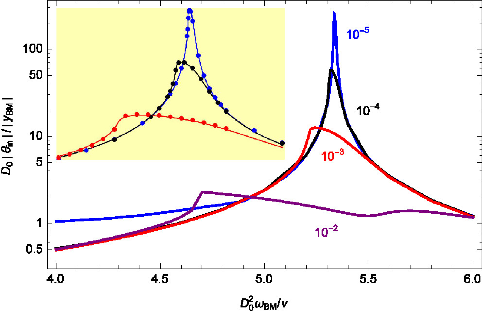
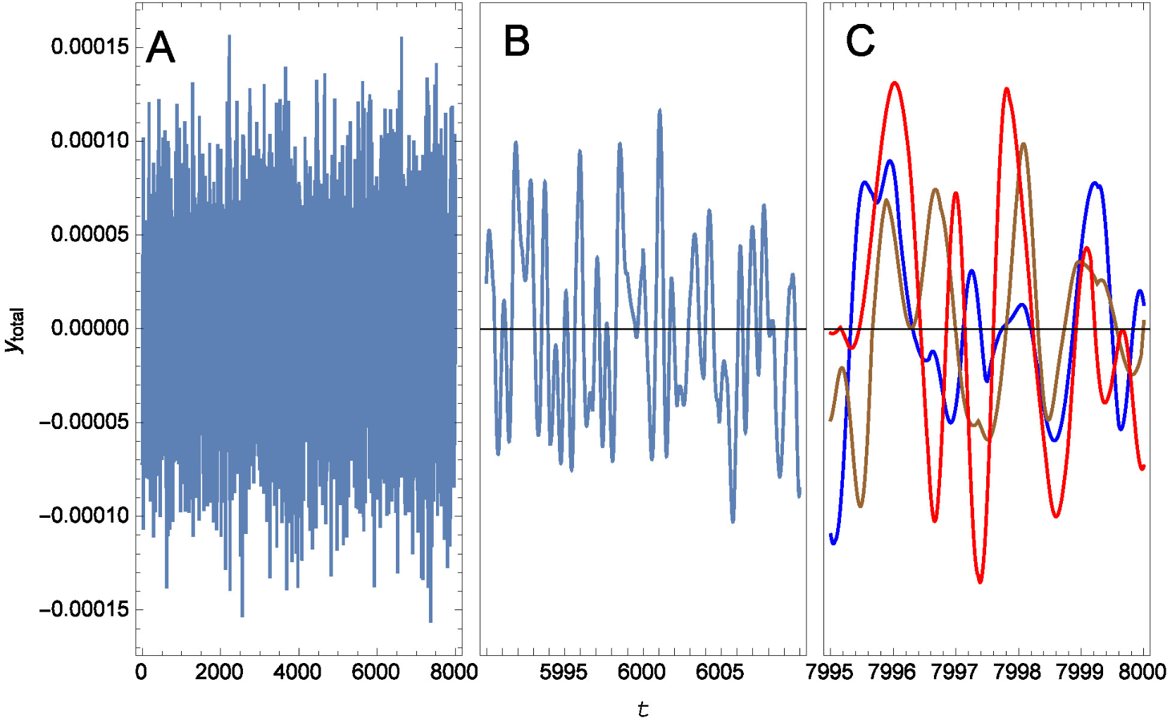
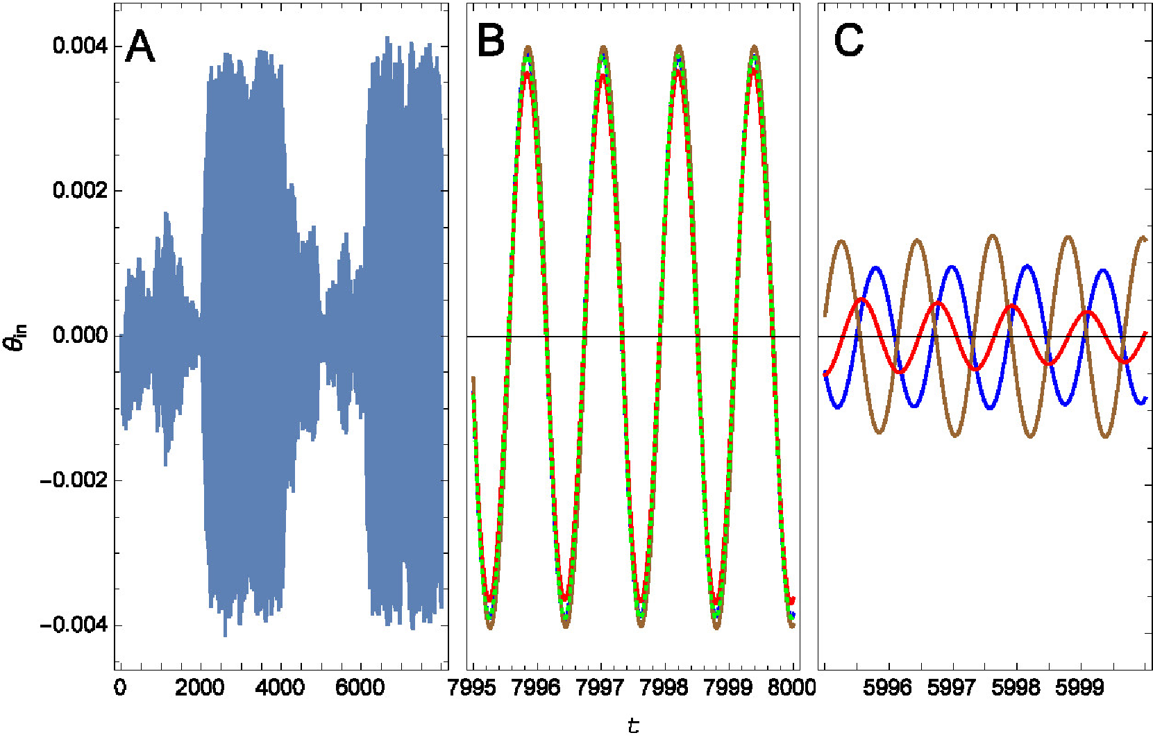
The article contains four appendices that include (1) generalization of the phase-lag concept to non-sinusoidal functions, (2) extension of Poiseuille’s equation (flow-pressure relation) to non-stationary boundaries, (3) input-output dependence near a Hopf bifurcation and (4) differentiation between amplification in the cochlea along distance or along time.
The cells below provide the most common calculations required and they closely follow the definitions in the article. If you run into any difficulty, you are welcome to contact the authors.
Geometric parameters
Geometric parameters
L=10;(*lengthofRL*)LH=10;(*lengthofHC*)LT=L+0.5LH^2/(L+LH);(*lengthofTM*)x1=3;(*centerof1stOHC*)x2=7;(*centerof2ndOHC*)ell=2;(*extensionofOHCinradialdirection*)
Dynamic parameters
Dynamic parameters
m=10;(*massateachendofanOHC*)mH=120;(*massofHC*)IRL=2.*^3;(*momentofinertiaofRL*)KRL=1.*^3;(*torsionalspringconstantonRL*)KCP=1.*^2;(*springconstantbetweenRLandCP*)betaCP=3;(*dampingconstantbetweenRLandCP*)KC=50;(*springconstantbetweenendsofOHC*)betaC=43;(*dampingconstantbetweenendsofOHC*)DEL=0.25375;(*maximumcontraction*)KD1=4.*^2;(*springconstantbetween1stDCandBM*)KD2=4.*^2;(*springconstantbetween2ndDCandBM*)beta1=3;(*damping1stDC*)beta2=3;(*damping2ndDC*)beta12=3;(*frictionbetweenDC1-2*)KB=10;(*springconstantouterbundles*)H1=6.5*^-3;(*extensionunstablerangeOHB1*)H2=5.*^-3;(*extensionunstablerangeOHB2*)KIHC=10;(*torsionalspringconstantinnerbundle*)HIN=5.*^-3;(*extensionsoftrangeIHB*)cs=2;(*innersulcusresistancetocompression*)mu=10;(*dragcoefficientIHB*)amp=310^-5;(*inputamplitude*)wbm=5.3294;(*inputangularfrequency*)noise=2.*^-6;(*representativevaluefor2k_BT/thickness*)
Variables
Variables
q: Q(0, t); tet: θ; b1: ; b2: ; s1: ; s2: ; tin: ; pin:
wn1, wn2, wn3, wn4: noise frequencies
ph1, ph2, ph3, ph4: noise phases
b
1
b
2
s
1
s
2
θ
in
p
in
wn1, wn2, wn3, wn4: noise frequencies
ph1, ph2, ph3, ph4: noise phases
Initial values
Initial values
(*Letter"p"standsfortimederivativeand"0"forinitialvalue*)tet0=RandomVariate[NormalDistribution[0,Sqrt[noise/KRL]]];tetp0=RandomVariate[NormalDistribution[0,Sqrt[noise/IRL]]];b10=RandomVariate[NormalDistribution[0,Sqrt[noise/KCP]]];b1p0=RandomVariate[NormalDistribution[0,Sqrt[noise/m]]];b20=RandomVariate[NormalDistribution[0,Sqrt[noise/KCP]]];b2p0=RandomVariate[NormalDistribution[0,Sqrt[noise/m]]];s10=RandomVariate[NormalDistribution[0,Sqrt[noise/KD1]]];s1p0=RandomVariate[NormalDistribution[0,Sqrt[noise/m]]];s20=RandomVariate[NormalDistribution[0,Sqrt[noise/KD1]]];s2p0=RandomVariate[NormalDistribution[0,Sqrt[noise/m]]];pin0=RandomVariate[NormalDistribution[0,Sqrt[noisecs]]];q0=0;tin0=0;
Input
Input
x-dependence, forces and torques
x-dependence, forces and torques
Dynamic equations
Dynamic equations
Time integration
Time integration
Re-initialization for extension of follow up time
Re-initialization for extension of follow up time
Amplitude and phase
Amplitude and phase