ABSTRACT (original article): Climate change threatens global food security. Mitigating this threat requires developing agricultural varieties that are resistance to pests and resilient to extreme conditions, such as drought. Improving resistance to drought and to some soil parasites is possible through synthetic biology and genome edition of plants. However, gathering whole plant, multi level, data to test the effects of genome interventions is inherently challenging because plants grow slowly, are time and resource consuming, and field experiments on testing the effectiveness of those interventions are laborious and may be difficult to perform. Mathematical models can be used to implement genome interventions in silico, simulate their effects, and prioritize the ones that are most likely to be effective for field testing.
Here, we present an example of how such multi level modeling can be done and used. We focus on the modulation of strigolactones (SLs) biosynthesis in maize and on the effects that changing their levels by manipulating the activity of various genes might have on maize root architecture. SLs are phytohormones that help a plant’s root to develop. They are also present in root exudates and induce germination of parasitic plant seeds, such as Striga and Orobanche. Here, we developed and analyzed a ODE-based mathematical model for the biosynthetic pathway of SLs, connected to a model that grows roots for individual maize plants in 3D. The model allows in silico testing of the effects of changing enzyme activities on SLs production, and how those change will affect root phenotypical characteristics such as length, lateral root branching, volume, and surface area. While we focus on SLs and maize roots, models for other molecular pathways could be implemented and plugged in. Modeling the above growth of the plant and coupling that growth to the other model is also fairly straight forward. CITATION (original article): Lucido A, Basallo O, Sorribas A, Marin-Sanguino A, Vilaprinyo E and Alves R (2022) A mathematical model for strigolactone biosynthesis in plants. Front. Plant Sci. 13:979162. https://doi.org/10.3389/fpls.2022.979162
Here, we present an example of how such multi level modeling can be done and used. We focus on the modulation of strigolactones (SLs) biosynthesis in maize and on the effects that changing their levels by manipulating the activity of various genes might have on maize root architecture. SLs are phytohormones that help a plant’s root to develop. They are also present in root exudates and induce germination of parasitic plant seeds, such as Striga and Orobanche. Here, we developed and analyzed a ODE-based mathematical model for the biosynthetic pathway of SLs, connected to a model that grows roots for individual maize plants in 3D. The model allows in silico testing of the effects of changing enzyme activities on SLs production, and how those change will affect root phenotypical characteristics such as length, lateral root branching, volume, and surface area. While we focus on SLs and maize roots, models for other molecular pathways could be implemented and plugged in. Modeling the above growth of the plant and coupling that growth to the other model is also fairly straight forward. CITATION (original article): Lucido A, Basallo O, Sorribas A, Marin-Sanguino A, Vilaprinyo E and Alves R (2022) A mathematical model for strigolactone biosynthesis in plants. Front. Plant Sci. 13:979162. https://doi.org/10.3389/fpls.2022.979162
Introduction
Introduction
Maize (Zea mays) is the most extensively cultivated cereal crop worldwide [1]. Parasitic plants, such as Striga or Orobanche [2], and climate change, with rising temperatures and more frequent droughts, can negatively impact maize production [3]. This impact can be partially mitigated by changing root architecture and creating root systems that grow deeper and more branched, accessing additional water sources. Changing root architecture can be done by editing the genome of plants, as long as we understand the factors that control root growth and how variations in those factors can be used to optimize root architecture for better production efficiency in adverse conditions. Phytohormones, such as strigolactones, inhibit shoot branching and increase the length of primary and seminal roots [4]. In addition, increasing the amount of SLs present in root exudates stimulates Striga or Orobanche growth [2]. Therefore, either modulating the concentration of these hormones through genetic modification of their biosynthetic pathways or using chemical hormone analogs could be excellent root optimization strategies that increase maize production [5].
The architecture of maize roots evolved to increase plant efficiency in the uptake of water and nutrients and to provide soil anchorage. The morphology of a maize root system consists of [6]:
◼
a primary root, the first branch that grows from the seed.
◼
a variable number of seminal roots that start to form when seed germinates and at the beginning of plant growth.
◼
a variable number of crown roots, shoot borne roots that grow below ground.
◼
a variable number of brace roots, another shoot borne type of roots that initiate their growth aboveground, and then penetrate the soil.
◼
a variable number of secondary root branches called lateral roots, that grows along the main root axes branches.
A maize plant takes about sixty days to grow and typical weather conditions support one plant growth cycle a year [7]. Testing the effect that different interventions might have on root architecture can be exceedingly slow. Creating multilevel mathematical models that can be used to simulate and predict that effect can significantly speed up the development of new, more resistant, plant strains. These models enable the simulation of root growth under alternative conditions and permit evaluating the effect those conditions on specific and important root parameters, without the a priori need for real plant growth [8] . The versatility of Mathematica, where we could seamlessly integrate molecular, cellular, and whole organism simulations, makes it an ideal environment to create, simulate and analyze such multi level models. Here we present a two-level model that can be used to simulate the effect of changing gene activity on the biosynthesis of SLs, as well as the effect of changing SLs levels on the growth of realistic root architectures for individual maize plants.
How strigolactones are produced?
How strigolactones are produced?
The pathway for the biosynthesis of the two types of strigolactones - strigol-type and orobanchol-type.
The pathway for the biosynthesis of the two types of strigolactones - strigol-type and orobanchol-type.
Healthy plants produce SLs from all-trans-β-carotene (BCAR), through a multistep biosynthetic pathway [5]. Hereafter we assume that the plant is able to maintain the homeostasis of BCAR, by producing it at a constant rate. The key steps in the SLs biosynthesis pathway in maize are as follows:
◼
Step 1 - Conversion of BCAR to CISB: a β-carotene isomerase converts BCAR to 9-cis-β-carotene (CISB). This reaction is reversible.
◼
Step 2 - Cleavage of CISB: a carotenoid cleavage dioxygenase cleaves CISB into all-trans-β –apo-10′-carotenal (CTNL) and β –ionone.
◼
Step 3 - Conversion of CTNL to CL: a P450 enzyme converts CTNL into carlactone (CL).
◼
Step 4 - Conversion of CL to CLA: a P450 enzyme converts CL to carlactonic acid (CLA).
◼
Step 5 - Conversion of CLA to DO: CLA is converted to 4-deoxyorobanchol (DO) by a P450 enzyme.
◼
Step 6 - Conversions of DO to ORO: DO is converted into orobanchol (ORO) by a P450 enzyme.
◼
Step 7 - Conversion of CLA to ORO: CLA is converted to ORO by a P450 enzyme.
◼
Step 8 - Conversion of CLA to SR: CLA is converted into a strigol (STR).
◼
Step 9 - STR and ORO are released to the environment in root exudates.
Mathematical modeling of the biosynthetic pathway of strigolactones.
Mathematical modeling of the biosynthetic pathway of strigolactones.
We can model the biosynthesis of STR and ORO using the following system of ODEs [5]:
dBCAR
dt
kcat1×BCAR
Km1+BCAR
kcat2×CISB
Km2+CISB
dCISB
dt
kcat1×BCAR
Km1+BCAR
kcat2×CISB
Km2+CISB
kcat3×CISB
Km3+CISB
dCTNL
dt
kcat3×CISB
Km3+CISB
kcat4×CTNL
Km4+CTNL
dCL
dt
kcat4×CTNL
Km4+CTNL
kcat5×CL
Km5+CL
dCLA
dt
kcat5×CL
Km5+CL
kcat5×CLA
Km5+CLA
kcat6×CLA
Km6+CLA
dDO
dt
kcat5×CLA
Km5+CLA
kcat5×DO
Km5+DO
dORO
dt
kcat5×DO
Km5+DO
kcat6×CLA
Km6+CLA
dSTR
dt
kcat6×CLA
Km6+CLA
Values for the various constants and dependent variables can be taken from [5]:
In[]:=
ssrf=10^-4;ssri=10^-10;DepVars={BCAR,CISB,CTNL,CL,CLA,DO,ORO,STR};parameterValues={k010^-8,kcat168*1.07*10^-7,kcat234*1.07*10^-7,Km10.26,Km20.26,kcat32.6*1.07*10^-3,Km30.0087,kcat40.18*1.06*10^-6,Km40.0092,kcat56.08*10^-6,Km55.*10^-4,kcat63.8*10^-9,Km60.016,kORO1,kSR1,ϕ0.5};SubDepVarsWithoutT={BCAR[t]BCAR,CISB[t]CISB,CTNL[t]CTNL,CL[t]CL,CLA[t]CLA,DO[t]DO,ORO[t]ORO,STR[t]STR};randomInitialConditions=Table[{DepVars[[k1]],Random[Real,{ssri,ssrf}],0,Infinity},{k1,1,Dimensions[DepVars][[1]]}];
We can define these equations in the following way:
In[]:=
rates={r1[t_,BCAR_]:=(kcat1*BCAR)/(Km1+BCAR),r2[t_,CISB_]:=(kcat2*CISB)/(Km2+CISB),r3[t_,CISB_]:=(kcat3*CISB)/(Km3+CISB),r4[t_,CTNL_]:=(kcat4*CTNL)/(Km4+CTNL),r5[t_,CL_]:=(kcat5*CL)/(Km5+CL),r6[t_,CLA_]:=(kcat5*CLA)/(Km5+CLA),r7[t_,CLA_]:=(kcat6*CLA)/(Km6+CLA),r8[t_,DO_]:=(kcat5*DO)/(Km5+DO)};
In[]:=
ode={[t]ko-r1[t,BCAR[t]]+r2[t,CISB[t]],[t]r1[t,BCAR[t]]-r2[t,CISB[t]]-r3[t,CISB[t]],[t]r3[t,CISB[t]]-r4[t,CTNL[t]],[t]r4[t,CTNL[t]]-r5[t,CL[t]],[t]r5[t,CL[t]]-r6[t,CLA[t]]-ϕ*r7[t,CLA[t]]-(1-ϕ)*r7[t,CLA[t]],[t]r6[t,CLA[t]]-r8[t,DO[t]],[t]ϕ*r7[t,CLA[t]]+r8[t,DO[t]]-kORO*ORO[t],[t](1-ϕ)*r7[t,CLA[t]]-kSR*STR[t]};
′
BCAR
′
CISB
′
CTNL
′
CL
′
CLA
′
DO
′
ORO
′
STR
In[]:=
rateEquations=Join[ode][[All,2]]/.SubDepVarsWithoutT/.FilterRules[parameterValues,Except[ko]];
Effects of modulating β-carotene on strigolactones production
Effects of modulating β-carotene on strigolactones production
Experimentally, we can modulate the production of β-carotene by manipulating the genome of maize. The model reproduces this modulation by changing k0. As such, we can simulate the effect of synthesizing different amounts of β-carotene on the production of STR and ORO by scanning the values of k0 and calculating the corresponding steady state values for the dependent variables of the model.
In[]:=
rootSolution=Table[Join[FindRoot[(rateEquations/.{ko10^i})0,Table[{DepVars[[k1]],Random[Real,{ssri,ssrf}],0,Infinity},{k1,1,Dimensions[DepVars][[1]]}]],{ko10^i}],{i,-10,-6,0.01}]//Quiet;
We can now plot how changing k0 changes ORO and STR
In[]:=
OROSTR=ListPlot[{Table[{Log10[rootSolution[[j,9,2]]],Log10[rootSolution[[j,8,2]]]},{j,1,Dimensions[rootSolution][[1]]}],Table[{Log10[rootSolution[[j,9,2]]],Log10[rootSolution[[j,7,2]]]},{j,1,Dimensions[rootSolution][[1]]}]},ImageSize250,PlotRangeAll,AxesFalse,PlotLegends{"STR","ORO"},FrameTrue,FrameLabel{Style[Text[" (mM/s)"],FontFamily"Arial",FontColorBlack,FontSize12,FontWeightBold],Style[Text["Log[Concentrations]"],FontFamily"Arial",FontColorBlack,FontSize12,FontWeightBold]},FrameStyle{Thick},FrameTicks{{All,None},{All,None}},FrameTicksStyleDirective[Black,"Arial",12],PlotStyle{{PointSize[0.01],Red},{PointSize[0.01],Blue}}]
k
0
Out[]=
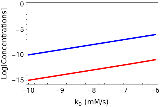


Figure 1: Effect of changing the production of β-carotene on the production of STR and ORO.
We can also study the effect of k0 on the stability of the steady state by plotting how the least negative real part of all the eigenvalues changes as a function of k0:
In[]:=
maxeig=Map[Max,Re[Map[Eigenvalues,Outer[D,rateEquations,DepVars]/.rootSolution]]];STAB=ListPlot[Table[{Log10[rootSolution[[j,9,2]]],Log10[-maxeig[[j]]]},{j,1,Dimensions[rootSolution][[1]]}],ImageSize250,PlotRangeAll,AxesFalse,JoinedTrue,FrameTrue,FrameLabel{Style[Text[" (mM/s)"],FontFamily"Arial",FontColorBlack,FontSize12,FontWeightBold],Style[Text["LogMax[-Re[λ]]]"],FontFamily"Arial",FontColorBlack,FontSize9,FontWeightBold]},FrameStyle{Thick,FontFamily"Arial",FontColorBlack,FontSize9,FontWeightBold},FrameTicks{{All,None},{All,None}},FrameTicksStyleDirective[Black,"Arial",12],PlotStyle{{PointSize[0.01],Red},{PointSize[0.01],Blue}}]
k
0
Figure 2: Effect of changing the production of β-carotene on the least negative real part of all eigenvalues for the steady state of the SLs biosynthesis pathway.
Figure 2 shows that the least negative eigenvalue for the steady state is always negative, but that it can be arbitrarily close to zero at β-carotene production rates close to 10E-6.7. This is indicative that transient between steady states caused by sustained changes in the supply of β-carotene may be slow.
Building in silico 3D root system architecture
Building in silico 3D root system architecture
Building the root architecture for one maize plant
Building the root architecture for one maize plant
Each maize plant possesses a unique Root System Architecture (RSA), shaped by a combination of genetic factors, environmental stimuli, and stochastic events. To introduce variability in our model, we employ statistical distributions whose parameters are calculated from experimental data, drawing random values for the properties of the individual root strands from these distributions during each root simulation. This approach ensures that our root models exhibit statistical characteristics akin to real plants.
We start building one RSA by randomly selecting its properties from the distributions mentioned in the previous paragraph, and predefine the temporal granularity for building the root. The model comprises four modules corresponding to primary, crown, seminal, and brace roots. Commencing with the primary root, we proceed to ascertain the quantities of crown, seminal, and brace roots using the relevant distributions for each root type. The algorithms for crown, seminal, and brace root modules are analogous, with the primary root module diverging by lacking branching.
The initial step of the algorithm involves establishing the origins of all roots, assuming level ground at coordinates (0, 0, 0). Primary and seminal roots initiate growth at or below the z-coordinate 0, while shoot-borne/nodal roots are categorized as brace roots if above ground or crown roots if below ground. Maize typically exhibits two above-ground whorls of brace roots and up to six below-ground whorls of crown roots. The distribution of whorl distances from [14] informs the selection of distances between whorls for maize roots, denoted as w_d. Consequently, the initial point of a brace root is either (0, 0, w_d) or (0, 0, 2×w_d), and the z-coordinate of the initial point of a crown root is randomly chosen from 0, -w_d, -2×w_d, -3×w_d, -4×w_d, or -5×w_d. Next, the length of each root strand is randomly generated based on the relevant statistical distribution. Axial angles are randomly chosen to determine the direction of the point subsequent to the root strand’s origin. The distance between successive points in a root strand is determined using an elongation function (see below), influenced by time after germination, length variability, and the impact of SLs. Finally, lateral roots are generated for each main root strand. Utilizing bootstrapping, we generate one thousand samples for the number of branches emerging from each strand and use the median value as the maximum potential number of lateral roots. A piecewise stochastic function decides whether lateral root branching occurs at each potential point, and if branching occurs, another stochastic function determines when its growth ceases. Below we present the mathematical functions and statistical distributions that are used in each step.
Mathematical implementation
Mathematical implementation
Root elongation
Root elongation
Initially, we establish a function that utilizes a point and angles to determine the subsequent point toward which the root will extend. This iterative process is repeated until the strand reaches its full growth. The root elongation and branching are governed by a set of rules. A single root strand, denoted as P = {P_1, P_2, ..., P_n}, grows from the initial point P_0 = (x_0, y_0, z_0) to the endpoint P_n = (x_n, y_n, z_n) within a 3-dimensional space. Equation (1) is employed to calculate the coordinates (x_i, y_i, z_i) of point P_(i>0):
The expression (cos A cos B) defines the x-coordinate (x_i), (cos B sin A) defines the y-coordinate (y_i), and (-sin B) defines the z-coordinate (z_i) governing the elongation direction of the root strand. These coordinates are determined based on the axial angles A and B. Axial angle A is randomly assigned within the range of 180° to 360°, while axial angle B is randomly assigned within the range of 0° to 180°.
The elongation function EF, specified in Equation (2), is employed to compute the length of a root strand at time t_i. Here, t_i is calculated as t_i = i/n t_f, where i represents the iteration number, n is the maximum number of iterations, and t_f is the final time.
The elongation function EF, specified in Equation (2), is employed to compute the length of a root strand at time t_i. Here, t_i is calculated as t_i = i/n t_f, where i represents the iteration number, n is the maximum number of iterations, and t_f is the final time.
Root branching
Root branching
Lateral roots emerge from primary, seminal, crown, and brace roots. Experimental measurements focus on quantifying lateral root branches per centimeter of the axis root. Jia et al. [16] observed variations in lateral root numbers per centimeter for different main root types, a consideration incorporated into our Root System Architecture (RSA) model. To simulate branching in a root strand, we initiate the process by generating a random number from the relevant distributions (see below). This number is then multiplied by the length of the strand, yielding the maximum potential number of branches {Br_1, Br_2, ..., Br_m} within that strand. Each Br_p represents a point in 3D space.
Eq (5) shows the lateral root function (LRF) that stochastically decides if a lateral branch will be formed or not. This is done by generating a random number and comparing that number by the probability of branching SBT. Lateral root branching hinges on the comparison between P(L_p) and the stop branching threshold (SBT), where SBT is determined by the product of the median (MedL) and the lateral root branching effect (Eq 4). MedL represents the median value derived from 1000 randomly generated values.
If P(L_p) - SBT<0, Br_p will connect to the set of points L_p. The length of the lateral root, L_p, is determined by the piecewise function in Eq (7). This equation is employed to compute both the probability of lateral root growth, P(L_pq), and the lateral root growth threshold (LRGT).
Here, P(L_pq) is randomly generated between 0 and 1, while LRGT is a random value between 0.4 to 0.9, simulating biological variability in lateral root formation. If P(L_pq)- LRGT≥0, the root stops growing. Otherwise, it will continue its growth. The points in lateral root L_p are defined as
where
Quantifying maize root morphology
Quantifying maize root morphology
Parameter values for the root models
Parameter values for the root models
First, we assigned parameter values for the various root parameters, based on measurements from [7]:
Modelling the growth of a single root system architecture
Modelling the growth of a single root system architecture
By comparing the various measurement tables below, we can see that each roots is quite similar to the other two, yet different. This reproduces the individual biological variation that plant biologists observe in their field experiments.
Table 1: Summary of the properties for the first in silico RSA. These properties are typically measured in field experiments.
Table 2: Summary of the properties for the second in silico RSA. These properties are typically measured in field experiments.
Table 3: Summary of the properties for the third in silico RSA. These properties are typically measured in field experiments.
We can further see the differences between roots by representing them visually. We start by creating a function that performs that representation.
We then use the function to represent the three roots:
Figure 3: A set of three individual wild type roots built using basal levels of SLs. The figure show that the same initial conditions leads to different root system architectures.
Modelling and analyzing the properties of a population of root system architectures: in silico “shovelomics”
Modelling and analyzing the properties of a population of root system architectures: in silico “shovelomics”
Usually, in the field, a large number of roots are collected and their properties are measured, in an approach that is colloquially known as “shovelomics”. To perform in silico “shovelomics” we can scale up the in silico experiment shown above. First we will look at how we can model several roots under similar conditions. Then we will investigate the effect of adding various amounts of SLs to the soil on the RSA of maize. We will perform a control experiments with no added SLs, where we will grow 20 individual maize RSAs. Then we will add increasing amounts of SLs to the soil and, for each amount check the RSA properties of the 20 RSA grown under those conditions. To do this we will create functions that can be used to perform the experiments. This function will have as input parameters the end time for the simulation of each RSA, the number of iterations for each simulation, the range of SLs concentration to add to the soil and the step in increasing SLs concentrations, and the number of roots to simulate for each concentration.
Modelling and analyzing several root system architectures
Modelling and analyzing several root system architectures
We will now perform the simulations for two values of SLs: 0 and 1 mM. The end time for the simulation of each RSA will be 40 day. The number of iterations for each simulation will be 150. The range of SLs concentration to add to the soil will be set between 0 and 2, and the step in increasing SLs concentrations will be 0.5. We will simulate 10 RSA per concentration.
Table 4: Summary of the properties for ten independent in silico RSA, grown with addition of 1mM external SLs. These properties are typically measured in field experiments.
Typically, the dataset of roots is analyzed with respect to various parameters: median number of the different types of roots, median length, branching density, and root depth [7]. Our in silico dataset can also be analyzed with respect to these parameters too.
Modelling the effect of changing strigolactone levels on root system architectures
Modelling the effect of changing strigolactone levels on root system architectures
When the user is interested in studying the statistical distribution of root variables under a given set of conditions, s/he can use MaizeRootAllData. The function requires four input variables: time in days, maximum number of iterations, number of roots, and strigolactone concentration. Then, MaizeStatsPlots can be used to perform the statistical analysis of the data, as shown in Table 1.
Figure 3: Summary of the effect of changing SLs concentrations on RSA.
Summary and Conclusion
Summary and Conclusion
To summarize, we present a maize modeling methodology, that integrates metabolism with macroscopic root growth, accounting for biological variability of individual plants, simulates the growth of individual root system architectures, represents those RSAs, and enables the statistical analysis of their properties. We extend the model to include functionality that can simulate and analyze the effect of the plant development hormones SLs on RSA. While we focus on SLs, incorporating other influences in the model should not be problematic using similar approaches.
The package has the potential to be adapted for other grain plants by gathering data from the literature.
The package has the potential to be adapted for other grain plants by gathering data from the literature.
References
References
◼
[1] Ranum, P., Peña, J. P., Peña-Rosas, P., Garcia-Casal, M. N. & Nieves Garcia-Casal, M. Issue: Technical Considerations for Maize Flour and Corn Meal Fortification in Public Health Global maize production, utilization, and consumption. Ann. N.Y. Acad. Sci doi:10.1111/nyas.12396.
◼
[2] Cook, C. E., Whichard, L. P., Turner, B., Wall, M. E. & Egley, G. H. Germination of Witchweed (Striga lutea Lour.): Isolation and Properties of a Potent Stimulant. Science 154, 1189-1190 (1966).
◼
[3] Tokatlidis, I. S. Adapting maize crop to climate change. Agron Sustain Dev 33, 63-79 (2013).
◼
[4] Ruyter-Spira, C. et al. Physiological effects of the synthetic strigolactone analog GR24 on root system architecture in arabidopsis: Another belowground role for strigolactones? Plant Physiol 155, 721-734 (2011).
◼
[5] Lucido, A. et al. A mathematical model for strigolactone biosynthesis in plants. Front Plant Sci 13, (2022).
◼
[6] Hochholdinger, F. The Maize Root System: Morphology, Anatomy, and Genetics. Handbook of Maize: Its Biology 145-160 (2009).
◼
[7] Boone,L. et al. Environmental life cycle assessment of grain maize production: An analysis of factors causing variability. Sci. Total Environ., 553, 551-564 (2016).
◼
[8] Lucido, A. unpublished doctoral dissertation, University of Lleida, (2023).
◼
[9] Arite, T., Kameoka, H. & Kyozuka, J. Strigolactone Positively Controls Crown Root Elongation in Rice. J Plant Growth Regul 31, 165-172 (2012).
◼
[10] Sun, H. et al. Strigolactones are involved in phosphate- and nitrate-deficiency-induced root development and auxin transport in rice. J Exp Bot 65, 6735-6746 (2014).
◼
[11] Zhu, J., Mickelson, S. M., Kaeppler, S. M. & Lynch, J. P. Detection of quantitative trait loci for seminal root traits in maize (Zea mays L.) seedlings grown under differential phosphorus levels. Theoretical and Applied Genetics 113, 1-10 (2006).
◼
[12] Liu, Z. et al. Enhanced crown root number and length confers potential for yield improvement and fertilizer reduction in nitrogen-efficient maize cultivars. Field Crops Res 241, (2019).
◼
[13] Jia, X., Liu, P. & Lynch, J. P. Greater lateral root branching density in maize improves phosphorus acquisition from low phosphorus soil. J Exp Bot 69, 4961-14790 (2018).
◼
[14] Liu, S., Sherard Barrow, C., Hanlon, M., Lynch, J. P. & Bucksch, A. DIRT/3D: 3D root phenotyping for field-grown maize (Zea mays). Plant Physiol 187, 739-757 (2021).
◼
[15] Leitner, D., Klepsch, S., Bodner, G., and Schnepf, A. A dynamic root system growth model based on L-Systems. Plant Soil 332, 177-192 (2010).
◼
[16] LJia, X., Liu, P., and Lynch, J. P. Greater lateral root branching density in maize improves phosphorus acquisition from low phosphorus soil. Journal of Experimental Botany 69, 4961-4970, (2018).
CITE THIS NOTEBOOK
CITE THIS NOTEBOOK
An example of multi-level modelling in plants
by Rui Alves
Wolfram Community, STAFF PICKS, March 22, 2024
https://community.wolfram.com/groups/-/m/t/3145876
by Rui Alves
Wolfram Community, STAFF PICKS, March 22, 2024
https://community.wolfram.com/groups/-/m/t/3145876