Quantum theory famously proves that the physical world governed by its rules can’t be simultaneously real and local. The Copenhagen interpretation simply admits defeat on the realism front, while other interpretations like Many Worlds and Superdeterminism try to hide it behind additional uncomfortable concepts such as the infinitudes of parallel universes and unexplained knowledge about the future. But all of these take locality as the absolute truth, never to be violated. The alternative is to concede that the world is non-local and one part of it can influence another instantaneously but still manage to preserve causality without breaking the sacred speed limit for any transfer of information. Bohmian mechanics is one such alternative, where particles always have definite properties, but these properties influence each other in a strange, non-local way.
In the traditional formulation of Bohmian mechanics, the only such definite property that particles have is their position in space. Any other properties, like mass, charge, and spin, are contextual, meaning they depend on the context of the measurement apparatus and the pilot wave guiding a particle through it. It argues that in the end, any measurement of such properties is inferred from some spatial indicators, like a dot on a screen, deflection in the non-uniform magnetic field in up or down direction or an actual arrow pointing to a calibrated gauge.
But nothing stops us from applying ideas of Bohmian mechanics to such properties, especially in the context of Quantum Computation. Discrete properties like spin or the state of a qubit are fundamentally different from the continuous position, meaning that it’s no longer possible to set up a deterministic differential equation of how they change. The equations have to be stochastic, which, unfortunately, would break another great achievement of the theory of removing the inherent non-determinism from its formulation, but keeps its promise of maintaining the realism with causality and as a result gives us a novel perspective to the nature of the quantum world.
Crash course on Bohmian mechanics
Crash course on Bohmian mechanics
Bohmian mechanics is simply an alternative interpretation of the Schrodinger equation:
Out[]=

(
1
)After writing the wave function in polar form:
Out[]=

(
2
)The Schrodinger equation splits into a continuity equation:
Out[]=

(
3
)And the Hamilton-Jacobi equation with a quantum potential:
Out[]=

(
4
)The combination of equations (3) and (4) form a Madelung fluid.
Particle interpretation of quantum hydrodynamics is developed under the formalism of stochastic quantum mechanics (Brownian motion with unspecified stochastic source).
Particle interpretation of quantum hydrodynamics is developed under the formalism of stochastic quantum mechanics (Brownian motion with unspecified stochastic source).
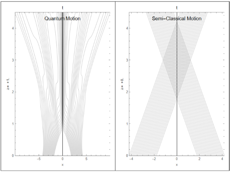
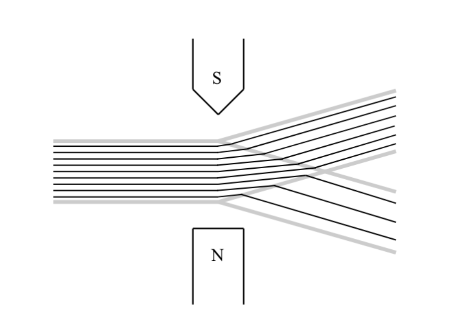
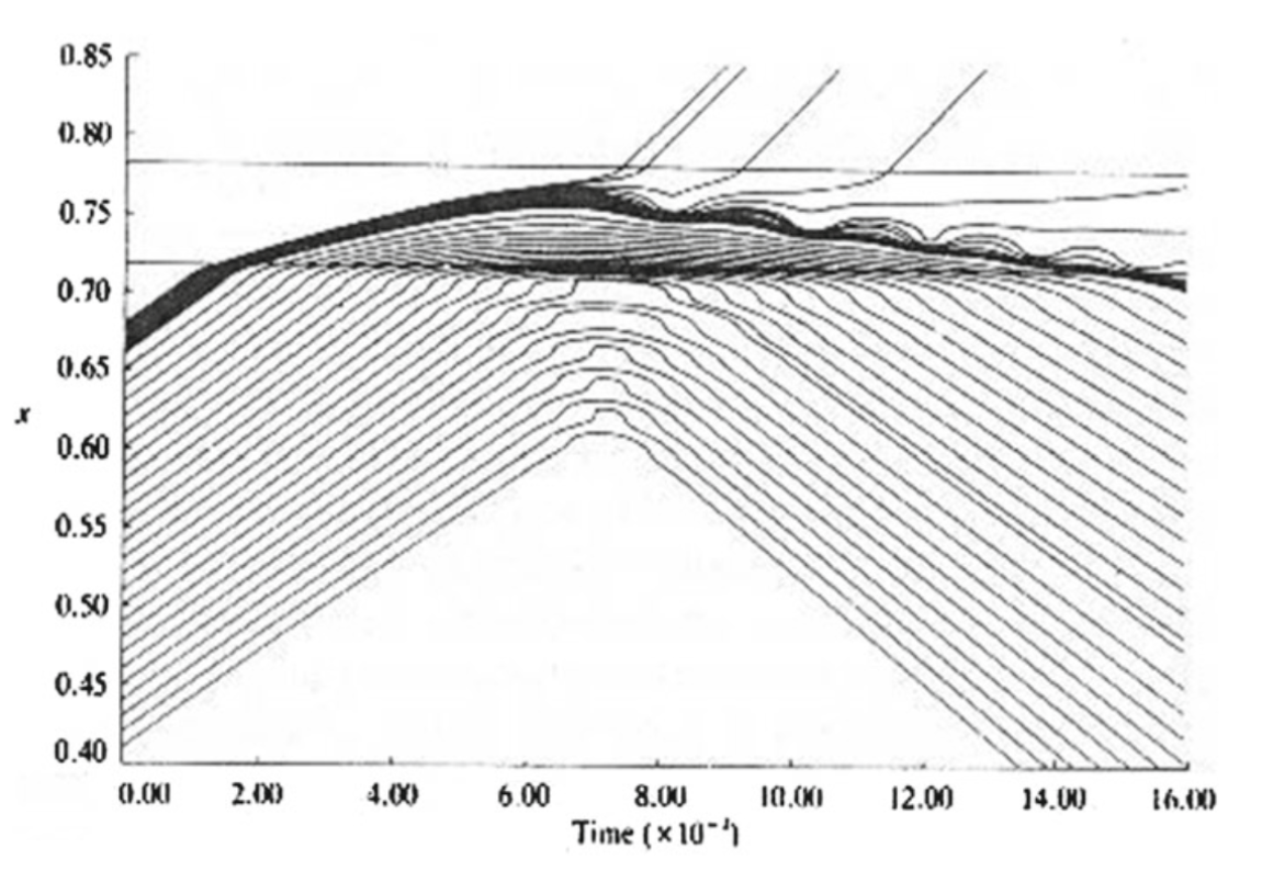
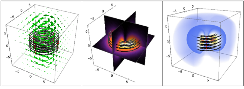
Hydrodynamic analogs produce a striking resemblance to famous quantum experiments.
Out[]=
Bohmian mechanics is a special case of stochastic mechanics, where quantum fluid particles no longer act as sources of the underlying field but assume a definite trajectory guided by the flow of the field (the pilot wave) without any back reaction from a particle onto the field.
Double-slit experiment
[1]
Stern-Gerlach experiment
[2]
Quantum tunneling
[3]
Hydrogen atom
[4]
Bohmian mechanics recovers both determinism and realism with trajectories as beables. The non-deterministic nature of quantum theory comes purely from our ignorance about the initial condition. All quantum properties like spin and energy levels are contextual, with values depending only on the real particle position and velocity together with measurement device settings.
Simple qubit
Simple qubit
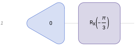
Let’s first consider a simple rotation of the basis state:
|0〉
In[]:=
<<Wolfram`QuantumFramework`
In[]:=
ρ0=QuantumState["0"];U=QuantumOperator["RX"[-Pi/3]];
Out[]=
Out[]=

Evolving the initial state using the Hamiltonian yields a smooth transition to the final state instead of a jump corresponding to the application of the rotation gate:
If one now thinks of the qubit as always being in the definite state, the probabilities at the final moment of evolution can be interpreted as qubit making a random jump from its initial basis state to its final basis state. As initial probabilities can also incorporate uncertainty about the qubit definite state, it doesn’t have to be deterministic, so both initial and final qubit states can be represented by probability vectors:
Of course, in the end it doesn’t matter which one is chosen, as all the statistics can be determined only from the initial and final probabilities alone. But if we want a more realistic intermediate view of the system guided by a definite probability current pushing the state from one basis state to another, we have to do better than that.
In general for a single qubit the current will always be of this form:
Where the frequency can be found directly from the Hamiltonian eigenvalues:
And coefficients can be determined from off-diagonal element of the initial and final (or any intermediate) density matrix:
Under this varying probability current, qubit’s probability density of transitioning also varies in time and is inversely proportional to the probability of being in the initial state, but only when the current is positive:
The integration capabilities of the Wolfram Language come to our rescue and we successfully compute the probability of the jump:
And because we’ve started from a definite 0 state, this would also correspond to the only possible way for the qubit ending up in state 1, which is also its exact final probability:
General qubit
General qubit
The general case is actually much more involved. Let’s consider a random unitary evolution of a random mixed qubit state:
Going through the same procedure of computing the probability current:
And the intermediate time varying probabilities:
The probability current now have a more complicated behaviour, crossing the x-axis multiple times, which means transition probabilities are switching between each other but still only allow for a single transition direction within each individual interval:
Now we need to compute transition probabilities for each interval separately by calculating the points where any of the curves cross the x-axis:
Then similarly to the simple example it is possible to assign a stochastic matrix to each individual interval by computing a bunch of integrals (numerically this time, as it is too complicated for analytic integration now) with appropriate changes depending on the sign:
The resulting single matrix is then computed by multiplying these three matrices together:
And we can confirm that the resulting matrix is indeed produces the desired dynamics of probabilities:
Packaging the above procedure into a single function results in the following:
Which makes it possible to compute the stochastic matrix for any qubit basis:
Non-locality and Contextuality
Non-locality and Contextuality
Why is it said that Bohmian mechanics is non-local, or how is it more common in modern times to call this feature of quantum theory contextual? In the computation case, it can be understood by considering the following example with an arbitrary entangled multi-qubit state and a single-qubit unitary acting on its part:
In order to compute its stochastic variant using the algorithm from the previous chapter, one should necessarily take into account all possible definite states for other parts of the system, or the following “context” states:
These states determine the stochastic evolution of the second qubit for each out of four possible contexts:
The stochastic matrices can then be assembled into a single multiplexer diagram for probabilities, effectively choosing which matrix to use based on the context:
Measurement problem
Measurement problem
Intermediate evolution of probabilities being in a definite state does not correspond to the Born probabilities (squared amplitudes) of the state itself:
Kolmogorov forward equation for a particle guided by the stream reproduces the probability density curve:
Of course it’s not enough to have a single such particle with discrete hidden value corresponding to a single basis. At least three such states are required in order to recover statistics from an arbitrary choice of measurement, and some additional interpretation is then needed for how these states project to a measurement basis and combine into a single outcome.
A solution to this may be an introduction of more qubit particles, in addition to a single one jumping between north and south pole of the Bloch sphere, each corresponding to a pair of antipodal states uniformly covering the sphere accounting for every possible measurement basis:
Given an initial probability distribution the location of these particles fully specify the quantum state:
Each pair now is guided by a different probability current and is subject to stochastic jumps along each direction:
The resulting stochastic dynamics of individual particles reproduces quantum state dynamics:
Multipartite system and Quantum Tomography
Multipartite system and Quantum Tomography
It is possible to represent multiple entangled qubits with just particles on their Bloch spheres in the same way, where corresponding definite states are correlated with each other:
We generate 2-qubit projectors for every direction with one aligned with the z-axis for simplicity:
And sample initial particles according to the joint distribution:
It is convenient to project spherical coordinates uniformly onto a plane to have a simple image of the quantum state:
Colors represent whether along a given direction particle is pointing up or down which depend on the direction qubit is being observed from:
These colored dots (bits) effectively represent a statistical micro-state of a qubit, with its usual complex amplitude and density matrix representations recovered using various tomography techniques.
Create a tomographic data with all the measurement operators and single measurement results:
Maximum likelihood estimate then produces a good approximation for the entangled state:
Linear inversion estimate:
Traced estimates:
Manual Maximum Likelihood estimation:
To estimate the conditional state vector along a given direction, sub-selection or weighting of directions is required:
The more subspaces there are, the more difficult it is to estimate the macro qubit state, for which the action of a gate is defined using a unitary or a Hamiltonian. With a fixed number of bit particles to statistically represent a qubit, the size of the system quickly partitions it into just a single bit per subspace, which would be insufficient to estimate the macrostate reliably. The amount of subspaces required to estimate an evolution of the macrostate depends on its purity with can be determined locally. For example maximally entangled GHZ states looks completely mixed everywhere locally, which means all the information is hidden in the correlation and all the induces subspaces are required to properly evolve each qubit:
Phase space picture
Phase space picture
An alternative way to represent a qubit state with a single definite trajectory is to perform a similar analysis in the phase space picture instead. We again take a random qubit evolution as an example:
But now instead of a density matrix and a Hamiltonian we would consider a probability vector and a quasi transition rate matrix (or Liouvillian with rows and columns summing up to 0) in the Symmetrically Information Complete (SIC) Tetrahedron basis:
The Tetrahedron basis is a measurement basis with POVM elements coinciding with the built-in polyhedron:
We can similarly evolve the probability vector and get the time-dependent probability vector:
And probability current having a much simpler form:
There is now a time-varying probability to jump between four different states, with always a fixed set of transitions being positive during the unit time interval of evolution:
The qubit’s trajectory consists of occupying one of four definite states at a single moment and jumping around with variable rates:
Because of multiple transitions it is now not so easy to compute the final stochastic matrix governing the evolution using precise integration (at least I’m not aware of the way to do it). Instead we do a simulation to confirm that the final probability is recovered from averaging over multiple simulation runs:
What we’ve essentially showed with that simulation, is that it is possible to render an underlying quasi-stochastic evolution as a time-dependent stochastic one. Which means that the solution to the following master equation (taking a very simple form in phase space) is a quasi stochastic matrix, matrix with rows summing up to 1 but with negative elements, but it can be simulated stochastically:
QBism and Markov chain Embedding Problem
QBism and Markov chain Embedding Problem
Any quasi-stochastic matrix can be decomposed into a product of commuting stochastic (forward) and inverse of stochastic (backward) matrices by simply shifting its values by the most negative element and rescaling:
The inverse of backward stochastic matrix can be thought of as applying Bayesian inference or following the Bayesian flow from a prior distribution to the posterior guided by the likelihood, which forms the basis for the QBist’s interpretation of quantum theory. Bayes rule can take multiple forms:
For the discrete case it can be more concretely written in index and vector notation:
With initial state playing the role of observations and is related to a final state by inverse of the backward stochastic map:
Many Bayesian steps are required to reach the posterior from any prior as though we’re moving across a gradient of some function:
But it is not clear how to construct the landscape function associated to the path produced by Bayesian updates, the more natural way to perform inference gradually is to follow the gradient field of the likelihood function:
For comparison here are the different trajectories starting from the same prior:
This quasi-stochastic matrix decomposition doesn’t guarantee a valid transition-rate matrix after taking a matrix logarithm of the above forward and backward components, which is known as the Markov chain Embedding Problem:
But if we take not the most negative probability as the shift but an arbitrary large negative value, then decomposition yields valid transition-rate matrices:
Quantum fluid in phase space
Quantum fluid in phase space
Instead the Liouvillian quasi transition-rate matrix can be decomposed directly to circumvent the Embedding Problem, which also would be analogous to the separation of streaming velocity of particles in the quantum fluid into its forward and osmotic parts:
This would produce another decomposition into forward and backward stochastic matrices:
But the convergence of the backward inference is much much slower:
Conclusion
Conclusion
◼
Qubits are represented as multiple discrete particles on a Bloch sphere or a single particle in tetrahedron phase space with stochastic dynamics governed by a current derived from arbitrary Hamiltonian.
◼
Non-locality of hidden variables is explicitly shown by constructing controlled stochastic matrices conditioned on other systems the qubit is entangled with.
◼
A unique choice of stochastic dynamics is derived from an assumption of qubit particles always having a definite value state at any moment.
◼
Connections to QBism and quantum Hydrodynamics are considered
Future Work
Future Work
◼
Quantum Computation as a limiting case of Hydrodynamic analogs with average zero position of a qudit particle
◼
Develop general quantum circuit simulator based on stochastic (hydro)dynamics
◼
...
References
References
1. Introduction to the Bohm-De Broglie Theory: The Causal Interpretation of the Quantum Theory
by Klaus von Bloh
Wolfram Community, STAFF PICKS, August 28, 2023
https://community.wolfram.com/groups/-/m/t/3000266
by Klaus von Bloh
Wolfram Community, STAFF PICKS, August 28, 2023
https://community.wolfram.com/groups/-/m/t/3000266
2. Norsen, Travis. 2013. “The Pilot-Wave Perspective on Spin.” arXiv [Quant-Ph]. arXiv. http://arxiv.org/abs/1305.1280.
3. C. Dewdney; B. J. Hiley (1982). A quantum potential description of one-dimensional time-dependent scattering from square barriers and square wells. , 12(1), 27–48. doi:10.1007/bf00726873
4. The Bohmian approach to the Hydrogen and Hydrogen-like atoms
by Klaus von Bloh
Wolfram Community, STAFF PICKS, October 5, 2023
https://community.wolfram.com/groups/-/m/t/3028340
by Klaus von Bloh
Wolfram Community, STAFF PICKS, October 5, 2023
https://community.wolfram.com/groups/-/m/t/3028340
5. Bell, J. S. n.d. “Beables for Quantum Field Theory.” https://informationphilosopher.com/solutions/scientists/bell/Beables_for_QFT.pdf.
6. Guerra, Francesco, and Rossana Marra. 1984. “Discrete Stochastic Variational Principles and Quantum Mechanics.” Physical Review D: Particles and Fields 29 (8): 1647–55.
CITE THIS NOTEBOOK
CITE THIS NOTEBOOK
Bohmian quantum computation: stochastic and causal interpretation of qubits
by Nikolay Murzin
Wolfram Community, STAFF PICKS, July 17, 2024
https://community.wolfram.com/groups/-/m/t/3223725
by Nikolay Murzin
Wolfram Community, STAFF PICKS, July 17, 2024
https://community.wolfram.com/groups/-/m/t/3223725