DesignModelFit linear model fit by design matrix
LinearModelFit for multivariate data by DesignMatrix
by Robert Nowak
LinearModelFit for multivariate data by DesignMatrix
by Robert Nowak
Suppose you want to fit a multivariate model via the DesignMatrix by LinearModelFit[] you will notice some information loss regarding the multivariate variables of the model.
Suppose we have sampled data points of a arc/circle/ellipse etc.
Lets generate some noisy elliptical bivariate test data t
Lets generate some noisy elliptical bivariate test data t
In[]:=
t=With{n=32},Table{2Cos@p,Sin@p}+RandomReal[.1{-1,1},2],p,0,2π-,;ListPlot[t,AspectRatioAutomatic,Frame->True]
2π
n
2π
n
Out[]=
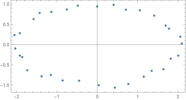
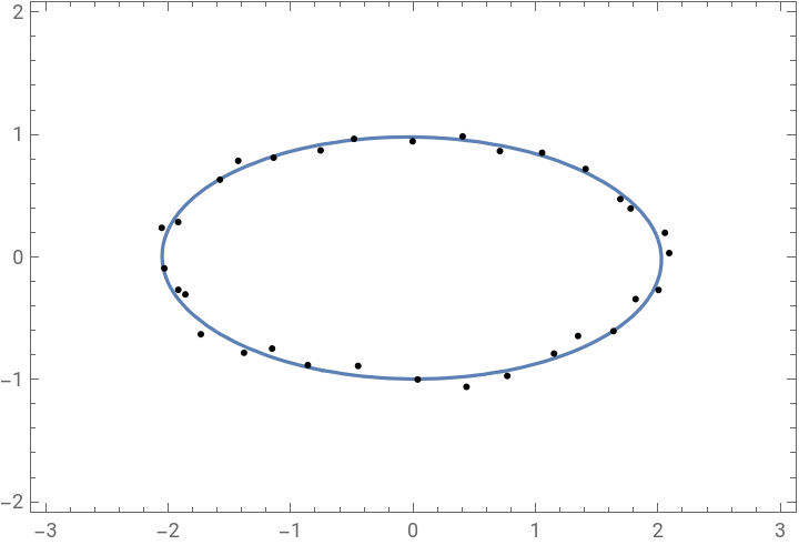
Lets perform a plain LinearModelFit lmf to get an algebraic fit of the data.
The fit model we choose is the general conic model mdl
This works as expected ;-).
The fit model we choose is the general conic model mdl
This works as expected ;-).
In[]:=
mdl={x,y,,,xy};lmf=LinearModelFit[t//Map[Append[1]],mdl,{x,y},IncludeConstantBasisFalse];lmf["BestFit"]//Labeled[#,"BestFit"]&//Framedlmf["BestFitParameters"]//Labeled[#,"BestFitParameters"]&//FramedContourPlot[lmf[x,y]1,{x,-3,3},{y,-2,2},AspectRatioAutomatic,EpilogPoint[t]]
2
x
2
y
Out[]=
Out[]=
Out[]=
Now we try to repeat the fit df via the DesignMatrix dm and the ResponseVector r.
In[]:=
dm=DesignMatrix[t//Map[Append[1]],mdl,{x,y},IncludeConstantBasisFalse];r=Table[1,Length@t];df=LinearModelFit[{dm,r},IncludeConstantBasisFalse];df["BestFit"]//Labeled[#,"BestFit"]&//Frameddf["BestFitParameters"]//Labeled[#,"BestFitParameters"]&//Framed
Out[]=
Out[]=
In[]:=
df["BestFitParameters"]lmf["BestFitParameters"]
Out[]=
True
As we can see, we get the same result in terms of “BestFitParameters”.
Unfortunately we have lost the information about the original two variables.
Now we are faced with five Slot parameters instead of two variables ;-(.
Unfortunately we have lost the information about the original two variables.
Now we are faced with five Slot parameters instead of two variables ;-(.
To overcome this inconvenience we define DesignModelFit[] a wrapper for LinearModelFit as well as some auxiliary functions.
DesignModelFit
DesignModelFit
implementation
implementation
Out[]=
Now we ready to use DesignModelFit[]
First we create the DesignModel List dm containing the four items:
{DesignMatrix, ResponseVector, expressions, variables}.
First we create the DesignModel List dm containing the four items:
{DesignMatrix, ResponseVector, expressions, variables}.
In[]:=
dm=DesignModel[t//Map[Append[1]],mdl,{x,y}];Length@dm
Out[]=
4
Now lets do the DesignMatrix fit dmf:
In[]:=
dmf=DesignModelFit[dm]
Out[]=
FittedDesignModelFittedModel,{x,y,,,xy},{x,y}
2
x
2
y
The original variables are preserved.
The fit is callable with two parameters as expected
The fit is callable with two parameters as expected
In[]:=
dmf["BestFit"]dmf["Function"]dmf[a1,a2]dmf[42,Pi]
Out[]=
0.0050368x+0.240401+0.0182574y+0.0147671xy+1.02258
2
x
2
y
Out[]=
0.0050368#1+0.240401+0.0182574#2+0.0147671#1#2+1.02258&
2
#1
2
#2
Out[]=
0.0050368a1+0.240401+0.0182574a2+0.0147671a1a2+1.02258
2
a1
2
a2
Out[]=
436.377
All “Properties” of LinearModelFit are preserved/adapted, the five Slot parameters are converted back to the two variables x, y.
In[]:=
dmf["BestFit"]dmf["Function"]dmf["ANOVATable"]
Out[]=
0.0050368x+0.240401+0.0182574y+0.0147671xy+1.02258
2
x
2
y
Out[]=
0.0050368#1+0.240401+0.0182574#2+0.0147671#1#2+1.02258&
2
#1
2
#2
Out[]=
DF | SS | MS | F-Statistic | P-Value | |
x | 1 | 0.00176808 | 0.00176808 | 0.232767 | 0.633368 |
y | 1 | 0.00420514 | 0.00420514 | 0.553603 | 0.463276 |
2 x | 1 | 21.1316 | 21.1316 | 2781.95 | 8.95874× -29 10 |
2 y | 1 | 10.6538 | 10.6538 | 1402.56 | 8.20849× -25 10 |
xy | 1 | 0.00357288 | 0.00357288 | 0.470367 | 0.498666 |
Error | 27 | 0.205091 | 0.00759595 | | |
Total | 32 | 32. | | | |