Abstract. Real quantum processors have sparse connectivity, while quantum error-correcting codes need parity checks that touch four or more qubits at once. Given the coupling graph of IBM's 27-qubit device ibmq_mumbai and a fixed qubit budget (9 data, 14 measurement, 4 idle qubits), we look for distance-3 codes that the hardware can measure natively, without SWAP gates. Rather than routing information with SWAP insertions, we follow a bridge approach, in which every check is measured in place through a connected set of auxiliary qubits. The search runs as a funnel: all 77,539 budget-conforming qubit placements are generated, two provably necessary conditions reduce them to 14,805, and a sweep over every Pauli assignment certifies that exactly 35 placements admit a distance-3 subsystem code. A final physical requirement, that every X check is measured by a direct two-qubit tower and every Z check through a connected auxiliary bridges, selects two placements, which realize the same code in two embeddings. This code is, operator for operator, the published heavy-hexagon [[9,1,3]] code, and the first embedding is the arrangement realized experimentally by Sundaresan et al. (2023).
Introduction: The problem (case [[5,1,3]] in IBM’s Falcon 7-Qubit processor)
Introduction: The problem (case [[5,1,3]] in IBM’s Falcon 7-Qubit processor)
In[]:=
Needs["Wolfram`QuantumFramework`"]
Logical quantum circuits are written as if any pair of qubits could interact. A physical quantum platform does not offer this freedom: two-qubit gates are available only between qubits that are connected in the coupling graph of the device. Since a logical circuit is not aware of the real connectivity that the physical device can support, it has to be mapped onto the hardware by Quantum Layout Synthesis algorithms, which decide where each logical qubit is placed and insert the routing operations that the connectivity demands. We want to exemplify this problem with a case from quantum error correction: the implementation of the [[5,1,3]] code on IBM’s Falcon 7-qubit processor.
The [[5,1,3]] code is the most basic quantum error-correcting code: it encodes one logical qubit into five physical qubits, the minimum number required to protect it against an arbitrary single-qubit error. We encode a state , with: The encoding is performed by the following circuit:
α|0〉+β|1〉α〉+β〉
|0
L
|1
L

Out[]=
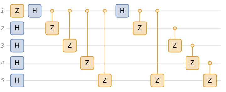
The five-qubit code is a stabilizer code whose stabilizer group is generated by the four operators . Measuring these generators does not read out the encoded state; instead, it extracts an error syndrome — a pattern of ±1 outcomes that identifies which error occurred on the data qubits. The syndrome extraction is implemented with the following circuit:
〈XZZXI,IXZZX,XIXZZ,ZXIXZ〉
Out[]=
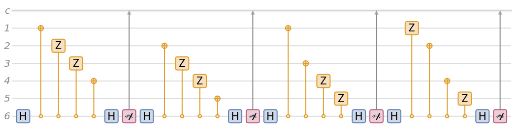
This construction needs the five physical qubits and one additional ancilla qubit, which allows us to read the errors indirectly. We measure the ancilla instead of the data, so the quantum information contained in the data qubits is not destroyed. As we can see, the ancilla qubit must interact with all five data qubits, so it would need to be connected to each of them. If an error occurs (let us say an X error on qubit 3) it anticommutes with some of the generators, and we can detect it by reading the syndrome:
In[]:=
Module[{ps0, psErr},
ps0 = PauliStabilizer["5QubitCode"]; psErr = ps0["X", 3];
Sign /@ Table[psErr["Expectation", g], {g, ps0["Stabilizers"]}]]
ps0 = PauliStabilizer["5QubitCode"]; psErr = ps0["X", 3];
Sign /@ Table[psErr["Expectation", g], {g, ps0["Stabilizers"]}]]
Out[]=
{-1,-1,1,1,-1}
The problem arises when, for example, we want to implement this circuit in a real quantum platform, such as the IBM’s Falcon 7-qubit processor, which qubits are connected according to the connectivity graph below.
Out[]=
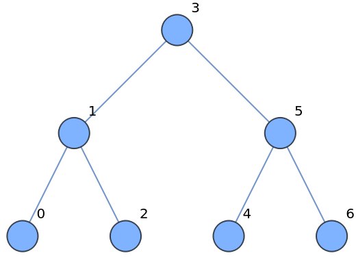
As we can see, with this connectivity there is no way to choose an ancilla qubit that is in contact with every data qubit. The standard solution is to insert SWAP operations when the circuit is transpiled to the real quantum platform. A SWAP gate moves the information stored in one qubit to a neighboring qubit, at the cost of three CNOT gates per SWAP (more gates = more noise). For this reason, the allocation of the ancilla qubits required by a QEC code is usually formulated as a layout-synthesis (qubit-mapping) optimization problem, which places the ancillas so that the number of SWAPs is reduced. For example:In this notebook, we explore a “bridge approach” to rediscover the heavy-hexagon [[9,1,3]] code on the IBM Mumbai 27-qubit processor.
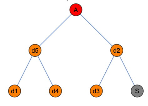
In the bridge approach, all data qubits remain at fixed vertices of the coupling graph , and each check with support is measured through a fixed set of auxiliary qubits , the ancilla bridge, chosen so that the induced subgraph on is connected and every qubit of is adjacent to at least one member of .
G(V,E)
P(S)
S
A
S
A
S
S
A
S
The bridge is prepared in an entangled (GHZ-type) state. Each of its qubits then accumulates, via CX or CZ gates, the parity of the data qubits it touches, and these partial parities propagate through the bridge so that a designated readout qubit ends up holding the eigenvalue of . Because errors on the data qubits still flip the recorded outcome in the same way as in a direct measurement, the bridged circuit preserves the error-detecting action of the original check, while the connectivity demand of a weight- operator is distributed over ancillas, each of which only needs its native degree. The costs are the extra ancillas and the additional two-qubit gates, roughly two per bridge link, compared with three per SWAP in routing-based methods.
±1
P(S)
w
A
S
Part 1: The IBM Mumbai 27-qubit processor
Part 1: The IBM Mumbai 27-qubit processor
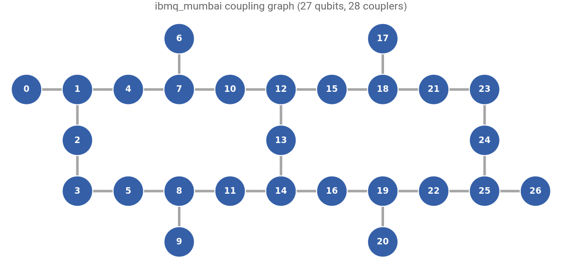
ibmq_mumbai is a 27-qubit superconducting quantum processor from IBM’s Falcon family. Its qubits are fixed-frequency transmons, connected by 28 couplers in a heavy-hexagon-inspired layout, and the native two-qubit gate is the CX (CNOT) gate. We take two inputs from this device: the coupling graph and the calibration data. Both come from FakeMumbaiV2 in qiskit-ibm-runtime, a snapshot of the real device’s reported properties.
ibmq_mumbai: 27 qubits, 28 couplers
Out[]=
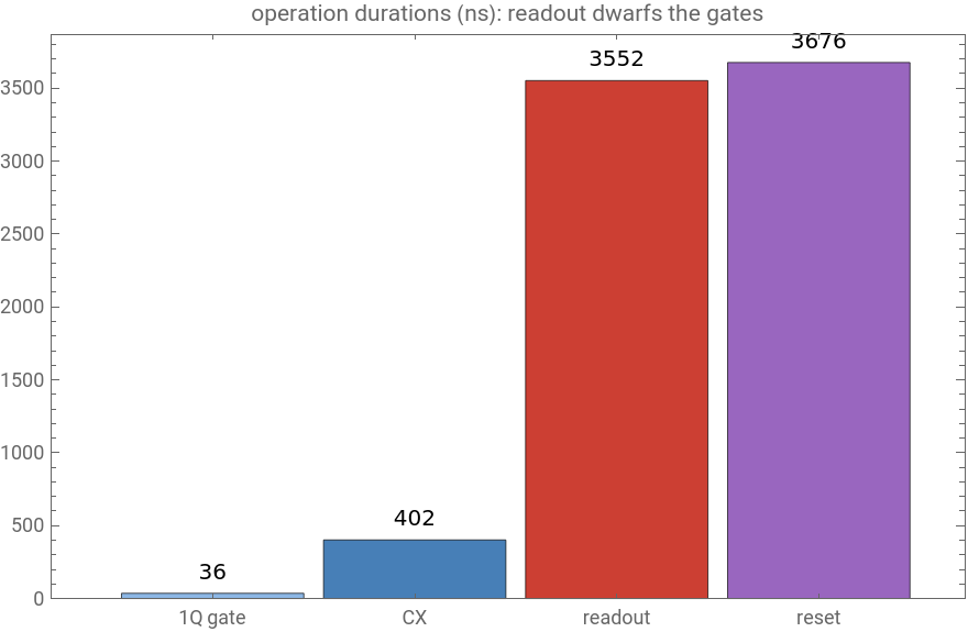
The chart below summarizes the calibration data that matters for this search. is the energy-relaxation time, the timescale on which a qubit decays from to ; is the dephasing time, on which a superposition loses its phase coherence. For this device, ≈ 112 μs and ≈ 124 μs. Against these clocks, a single-qubit gate takes 36 ns, a CX gate takes 402 ns, and the readout takes 3552 ns — nearly nine CX gates’ worth of time, during which every idle qubit simply decays. In addition, the readout flips the reported bit with probability 2.2%, and a CX gate fails with probability about 0.7%. These numbers, in particular the slow readout, will shape the economics of the code we search for.
T
1
|1〉
|0〉
T
2
T
1
T
2
Out[]=
coherence: T1 = 111.9 μs, T2 = 124. μs; readout flip probability 0.0216 |
For this device then, the search problem can be stated in one sentence: distribute the 27 physical qubits into three roles: 9 data qubits that store the code, 14 measurement qubits that extract syndromes, 4 idle qubits that rest; and find every role assignment that supports a distance 3 code. A role assignment is called a placement, stored as the pair {U, D} of unused and data qubits (the measurement set is the complement). The funnel below removes placements in stages and a stage may discard a placement only if the placement provably cannot complain the specified requirements.
≥
Part 2: Mumbai funnel: 77’539 → 14’805 → 35 → 2
Part 2: Mumbai funnel: 77’539 → 14’805 → 35 → 2
The Mumbai processor gives us 27 physical places, and the code needs three roles: 9 data qubits that store the logical information, 14 measurement qubits that extract the syndromes, and 4 idle qubits that remain unused. In this section, we enumerate every way to distribute the 27 qubits into these roles, and then we filter the resulting placements in three stages, following the funnel 77’539 → 14’805 → 35 → 2.
The search space. 77’539 placements
The search space. 77’539 placements
The device is the coupling graph {V,E} of Part 1, with qubits and couplers. A placement is a partition of the qubit set into three disjoint roles: a data set with , an unused set with , and the measurement (auxiliary) set formed by the remaining qubits. Since the measurement set is the complement of , a placement is completely specified by the pair .
G
H
|V|27
|E|28
D
|D|9
U
|U|4
27-4-914
U⋃D
{U,D}
In this subsection we need to impose two rules. First, the idle qubits are placed on pendant (degree-1) vertices, because idling an interior qubit destroys at least two couplers of usable wiring, while a pendant costs exactly one. Second, the 9 data qubits are required to be non-adjacent because syndrome extraction requires connections between data qubits and measurement or flag qubits, and in the fixed-data measurement model every interaction between data qubits must be mediated by measurement machinery.
In graph-theoretical language, the data qubits must form an independent set: , , and for every pair of distinct qubits and in . The implementation of this stage needs two short functions. pendants selects the degree-one vertices of the coupling graph, and lossOf counts the couplers that become unusable when a proposed set of four qubits is idled. The cell below applies lossOf to all possible four-qubit sets and finds that the minimum possible loss is four couplers, attained by selecting the four unused qubits from the pendant set . This motivates restricting the unused qubits to pendant locations.
D⊆V\U
|D|9
{u,v}∉E
u
v
D
17550
27 |
4 |
{0,6,9,17,20,26}
In[]:=
pendants=Select[Range[0,26],Length[nbrs[#]]==1&];lossOf[four_]:=28-Length[Select[edges,!IntersectingQ[#,four]&]];Row[{"minimum couplers lost over all ",Length[Subsets[Range[0,26],{4}]]," ways to idle four qubits: ",Min[lossOf/@Subsets[Range[0,26],{4}]]," achieved by choising the pendants: ",pendants,""}]
Out[]=
minimum couplers lost over all 17550 ways to idle four qubits: 4 achieved by choising the pendants: {0,6,9,17,20,26}
For each of the possible choices of unused pendant qubits, the recursive function indep searches the remaining qubits for every independent set of size 9 by backtracking: a candidate is added to chosen and all of its neighbors are removed from the remaining candidates, which guarantees that no later data qubit is adjacent to a previously selected one; a branch is stored when , and it is abandoned early if not enough candidates are left to reach nine. Sow records each valid pair and Reap collects all of them in allGeoms; the 14 measurement qubits are not stored explicitly because they are the complement of . The enumeration produces 77,539 valid placements.
15
6 |
4 |
|D|9
{U,D}
U⋃D
In[]:=
allGeoms=Reap[Do[Module[{avail=Complement[Range[0,26],unused],indep},(*backtracking*)indep[chosen_,cand_]:=If[Length[chosen]==9,Sow[{unused,chosen}],If[Length[chosen]+Length[cand]>=9,Do[indep[Append[chosen,cand[[i]]],Select[Drop[cand,i],!MemberQ[nbrs[cand[[i]]],#]&]],{i,Length[cand]}]]];indep[{},avail]],{unused,Subsets[pendants,{4}]}]][[2,1]];(*iddlequbits*)Row[{"4 pendant unused, 9 mutually non-adjacent data: ",Length[allGeoms]}]
First filter. 77’539 → 14’805 — measurable checks and two-check coverage
First filter. 77’539 → 14’805 — measurable checks and two-check coverage
In short, this filter demands that every data qubit is connected to at least two checks.
The function clusterOK rejects placements containing an auxiliary component that touches fewer than two or more than four data qubits. Finally, filtered selects from allGeoms the placements that pass clusterOK, offer between 3 and 14 candidate sites, and cover every data qubit at least twice, counting the coverage of each data qubit with:
Second filter. 14’805 → 35 (distance d ≥ 3)
Second filter. 14’805 → 35 (distance d ≥ 3)
Now suppose, as in an ordinary stabilizer code, that all measured checks commute. On a degree-3 graph the natively measurable checks are small (an auxiliary qubit reaches at most three data neighbors) and small commuting checks cannot build distance. However, in the subsystem construction (Poulin 2005) we can allow that the measured checks, now called gauge operators, are allowed to anticommute with each other; only suitable products of them (the center of the gauge group) must commute with everything. Those central products are the stabilizers, and they can have weight four or six even though every measured piece has weight two. Individual gauge outcomes are random (measuring an X-type gauge scrambles the anticommuting Z-type ones) but the stabilizer products are deterministic, which is why the scheme works.
Third filter. 35 → 2 (the heavy-hex measurement ansatz)
Third filter. 35 → 2 (the heavy-hex measurement ansatz)
This filter does not test the distance again. Instead, it asks which of the 35 algebraically valid arrangements can be measured using a swap-free, heavy-hex-inspired circuit family. This additional physical assumption reduces the list from 35 arrangements to 2.
Arrangements 10 and 20 realize the same abstract gauge-support pattern in two different physical embeddings of the Mumbai graph. Each of the other 33 arrangements fails because at least one X support lacks a direct tower, at least one Z support is classified as a tower, or both. Under the code-level relabeling symmetry used here, the two finalists represent the same abstract code, and both are the final results of this search. Finalist 1 (winner 10) is the arrangement that was realized experimentally by Sundaresan et al. (2023); finalist 2 (winner 20) remains an equally valid embedding under this model.
The important limitation is that the structural filter does not prove that the other 33 arrangements lack useful fault-tolerant measurement circuits. It proves only that they do not possess the particular direct-X, bridged-Z structure required by this heavy-hex-inspired ansatz.
Identifying the heavy-hexagon [[9,1,3]]
Identifying the heavy-hexagon [[9,1,3]]
Discussion and outlook
Discussion and outlook
Starting from only the coupling graph of ibmq_mumbai and a fixed budget of 9 data, 14 measurement and 4 idle qubits, a search found that exactly 35 of the 77,539 budget-conforming placements admit a distance-3 subsystem code; that a physically motivated measurement ansatz (direct two-qubit towers for X checks, auxiliary bridges for Z checks) reduces these to two placements, winners 10 and 20, which realize the same abstract gauge-support pattern in two embeddings; and that this pattern is, operator for operator, the published heavy-hexagon [[9,1,3]] code. Both finalists are final results of the search — no numerical ranking separates them in this structural model — and finalist 1 (winner 10) is precisely the arrangement that was realized experimentally by Sundaresan et al. (2023).
The constrains we imposed are: (1) The budget 9+14+4 is fixed, and it was chosen knowing that heavy-hexagon codes use nine data qubits, so other budgets are unexplored here. (2) Qubits are stationary: no SWAPs allowed. (3) Idle qubits sit on pendant vertices (defended by a counting argument) and data qubits form an independent set. (4) Every check is uniform-type (pure X or pure Z on its full support) so the search space is CSS by construction; non-CSS codes unexplored live on subgraphs of this very chip and are invisible to this sweep by rule. (5) The measurement is the heavy-hex-inspired: weight-two towers and bridges with data boundary two to four. Therefore the conclusion “exactly 35, then exactly 2” holds only inside our box.
The outlook and future work is clear: Replace the brute-force enumeration with a SAT solver, so we can escalate our approach to larger chips.Then use real per-qubit and per-coupler calibration (T1, T2, gate and readout errors) instead of solely geometric connectivity. Finally using other budgets (or not budgets), non-CSS checks, richer measurement gadgets, etc.
Acknowledgements
Acknowledgements
I would like to thank my mentor, Nikolay Murzin, for his support throughout the program, even from afar. I am also grateful to all the mentors and teaching assistants, who were always willing to help; every day and (quite) often at rather unreasonable hours. My thanks to Stephen Wolfram for making this program possible and for the conversations that turned into puzzles.
I would also like to thank my fellow participants for creating an environment in which simply walking through the common lounge could lead to unexpected discussions. Furthermore, thanks to Jhoan, whose apartment inadvertently became the program’s most productive nocturnal workspace. Finally, thank you to Laura, Pablo, Tigrann, Pedro, Montesinos, Curren, Matheo, and Alejandra for turning the long nights of work into some of the most memorable parts of the experience.
I would also like to thank my fellow participants for creating an environment in which simply walking through the common lounge could lead to unexpected discussions. Furthermore, thanks to Jhoan, whose apartment inadvertently became the program’s most productive nocturnal workspace. Finally, thank you to Laura, Pablo, Tigrann, Pedro, Montesinos, Curren, Matheo, and Alejandra for turning the long nights of work into some of the most memorable parts of the experience.
References
References
◼
D. Bacon (2006). Operator quantum error-correcting subsystems for self-correcting quantum memories. Physical Review A 73, 012340. arXiv:quant-ph/0506023.
◼
A. R. Calderbank, E. M. Rains, P. W. Shor and N. J. A. Sloane (1998). Quantum error correction via codes over GF(4). IEEE Transactions on Information Theory 44, 1369-1387. arXiv:quant-ph/9608006.
◼
C. Chamberland, G. Zhu, T. J. Yoder, J. B. Hertzberg and A. W. Cross (2020). Topological and subsystem codes on low-degree graphs with flag qubits. Physical Review X 10, 011022. arXiv:1907.09528.
◼
R. Chao and B. W. Reichardt (2018). Quantum error correction with only two extra qubits. Physical Review Letters 121, 050502. arXiv:1705.02329.
◼
M. Gong et al. (2022). Experimental exploration of five-qubit quantum error-correcting code with superconducting qubits. National Science Review 9, nwab011. arXiv:1907.04507.
◼
D. Gottesman (1997). Stabilizer Codes and Quantum Error Correction. PhD thesis, California Institute of Technology. arXiv:quant-ph/9705052.
◼
A. B. Khesin (2025). Quantum Computing from Graphs. PhD thesis, Massachusetts Institute of Technology. arXiv:2501.17959. Journal version: A. B. Khesin, J. Z. Lu and P. W. Shor, Universal graph representation of stabilizer codes, PRX Quantum 6, 040325 (2025), arXiv:2411.14448.
◼
L. Lao and C. G. Almudever (2020). Fault-tolerant quantum error correction on near-term quantum processors using flag and bridge qubits. Physical Review A 101, 032333.
◼
K. V. Milkevych, J. van de Pol and I. Shaik (2026). Practical subarchitectures for optimal quantum layout synthesis. Proc. 7th IEEE/ACM International Workshop on Quantum Software Engineering (Q-SE 2026). arXiv:2507.12976.
◼
D. Poulin (2005). Stabilizer formalism for operator quantum error correction. Physical Review Letters 95, 230504. arXiv:quant-ph/0508131.
◼
I. Shaik and J. van de Pol (2024). Optimal layout synthesis for deep quantum circuits on NISQ processors with 100+ qubits. 27th International Conference on Theory and Applications of Satisfiability Testing (SAT 2024). arXiv:2403.11598.
◼
N. Sundaresan, T. J. Yoder, Y. Kim, M. Li, E. H. Chen, G. Harper, T. Thorbeck, A. W. Cross, A. D. Corcoles and M. Takita (2023). Demonstrating multi-round subsystem quantum error correction using matching and maximum-likelihood decoders. Nature Communications 14, 2852. arXiv:2203.07205.
◼
K. Yin, H. Zhang, X. Fang, Y. Shi, T. S. Humble, A. Li and Y. Ding (2025). QECC-Synth: a layout synthesizer for quantum error correction codes on sparse hardware architectures. Proc. ASPLOS 2025. arXiv:2308.06428.
◼
Software and device data: Qiskit and qiskit-ibm-runtime fake providers (FakeMumbaiV2 coupling map and calibration snapshot); Wolfram Quantum Framework paclet (independent stabilizer cross-checks).
AI Disclosure
AI Disclosure
The following generative AI tools were used in this project: Claude Fable 5 by Anthropic. They were used for literature review, speed enhancement code, debugging, and editing prose. All code and written content was reviewed, understood and approved by the author.
CITE THIS NOTEBOOK
CITE THIS NOTEBOOK
Searching for d-3 Quantum Error Correcting Codes on a 27-qubit Superconducting Processor
by Luis Cervantes
Wolfram Community, STAFF PICKS, July 16, 2026
https://community.wolfram.com/groups/-/m/t/3763898
by Luis Cervantes
Wolfram Community, STAFF PICKS, July 16, 2026
https://community.wolfram.com/groups/-/m/t/3763898