We compute the LLE diagram and tie-lines for Water - Chloroform - Acetone at 25°C and 1 atm. Calculations use UNIQUAC activity coefficients and are based on a new approach, which is thoroughly described in Ref. 1-2.
Type I LLE ternary diagram for Water (1) - Chloroform (2) - Acetone (3) at 298.15 K and 1 atm
We use the UNIQUAC model in order to compute the activity coefficients.
We use the UNIQUAC model in order to compute the activity coefficients.
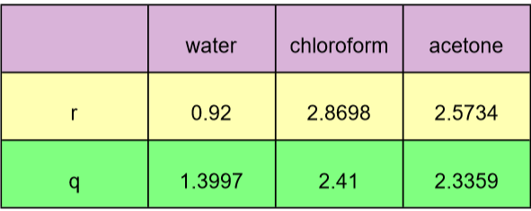
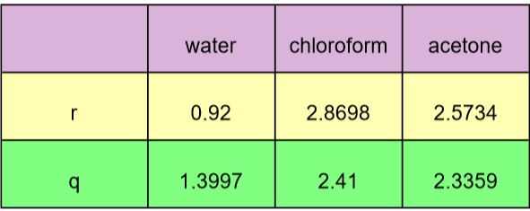
For the values of parameters r and q, they were taken from Aspen-HYSYS and they are reported in the Table below:
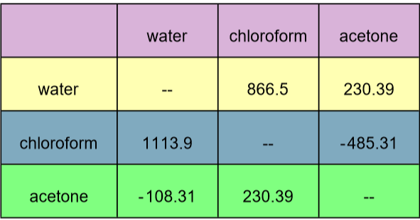
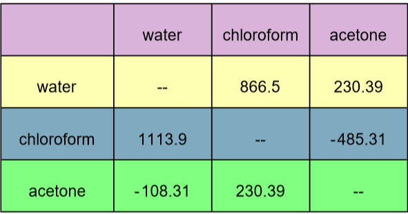
The binary interaction coefficients were computed using experimental data from Ref. 3 and a Matlab code for Particle Swarm Optimization. This PSO code yielded a root mean-square deviation (rmsd) equal to 2.057 % after 100 iterations and for a population size of 100. No further attempt was made to improve this value of the rmsd. Our calculated values (expressed in K) are given below :
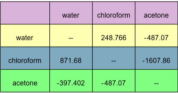
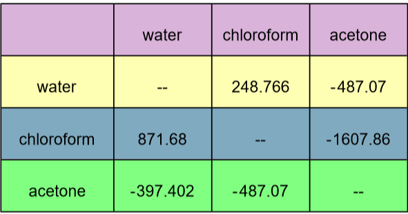
When the genetic algorithm approach (the command in Matlab is ga) was run using default options (maximum generation=100*6 and population size=50), the rmsd was slightly higher (rmsd=3.665 %). The corresponding values for the binary interaction parameters are reported in the Table below:In the present calculation, the set of parameters yielded by PSO was adopted.
In[]:=
TK=273.15+25;zc=10;tau[j_,i_]:=Exp[-t[j,i]];Gam1=Exp[Log[Gam1C]+Log[Gam1R]];Gam2=Exp[Log[Gam2C]+Log[Gam2R]];Gam3=Exp[Log[Gam3C]+Log[Gam3R]];Gam1C=ExpLog[phi[1]/x[1]]+zc2q[1]Log[v[1]/phi[1]]+l[1]-phi[1]x[1]x[j]l[j];Gam2C=ExpLog[phi[2]/x[2]]+zc2q[2]Log[v[2]/phi[2]]+l[2]-phi[2]x[2]x[j]l[j];Gam3C=ExpLog[phi[3]/x[3]]+zc2q[3]Log[v[3]/phi[3]]+l[3]-phi[3]x[3]x[j]l[j];Gam1R=Expq[1]1-Logv[j]tau[j,1]-v[k]tau[k,j];Gam2R=Expq[2]1-Logv[j]tau[j,2]-v[k]tau[k,j];Gam3R=Expq[3]1-Logv[j]tau[j,3]-v[k]tau[k,j];phi[i_]:=r[i]x[i]r[j]x[j];v[i_]:=q[i]x[i]q[j]x[j];GAMMA1=Gam1/.x[1]x1/.x[2]x2/.x[3]1-x1-x2;GAMMA2=Gam2/.x[1]x1/.x[2]x2/.x[3]1-x1-x2;GAMMA3=Gam3/.x[1]x1/.x[2]x2/.x[3]1-x1-x2;GAMMA1p=Gam1/.x[1]xp1/.x[2]xp2/.x[3]1-xp1-xp2;GAMMA2p=Gam2/.x[1]xp1/.x[2]xp2/.x[3]1-xp1-xp2;GAMMA3p=Gam3/.x[1]xp1/.x[2]xp2/.x[3]1-xp1-xp2;l[i_]:=zc/2(r[i]-q[i])-(r[i]-1);
3
∑
j=1
3
∑
j=1
3
∑
j=1
3
∑
j=1
3
∑
j=1
v[j]tau[1,j]
3
∑
k=1
3
∑
j=1
3
∑
j=1
v[j]tau[2,j]
3
∑
k=1
3
∑
j=1
3
∑
j=1
v[j]tau[3,j]
3
∑
k=1
3
∑
j=1
3
∑
j=1
In[]:=
r[1]=0.9200;q[1]=1.3997;r[2]=2.8698;q[2]=2.410;r[3]=2.57340;q[3]=2.3359;
In[]:=
Text@Style[Grid[{{"","water","chloroform","acetone"},{"r",r[1],r[2],r[3]},{"q",q[1],q[2],q[3]}},Frame->All,Background->{None,{Lighter[Blend[{Blue,Red}],.7],Lighter[Yellow,.7],{Lighter[Green,.5]}}},ItemSize->{1.5{5,4.2,4.2,4.2,5},3},Frame->Darker[Gray,.6],ItemStyle->14,Spacings->{1.3,.7}]]
Out[]=
In[]:=
t[1,3]=B13/TK;t[2,3]=B23/TK;t[1,2]=B12/TK;t[3,2]=B32/TK;t[3,1]=B31/TK;t[2,1]=B21/TK;t[1,1]=0;t[2,2]=0;t[3,3]=0;dd={1113.9,-108.31,866.5,230.39,400.66,-485.31};paramPSO={B12dd[[1]],B13dd[[2]],B21dd[[3]],B23dd[[4]],B31dd[[5]],B32dd[[6]]}
Out[]=
{B121113.9,B13-108.31,B21866.5,B23230.39,B31400.66,B32-485.31}
In[]:=
Text@Style[Grid[{{"","water","chloroform","acetone"},{"water","--",B21,B23},{"chloroform",B12,"--",B32},{"acetone",B13,B23,"--"}}/.paramPSO,Frame->All,Background->{None,{Lighter[Blend[{Blue,Red}],.7],Lighter[Yellow,.7],{Lighter[Blend[{Blue,Darker@Green}],.5],Lighter[Green,.5]}}},ItemSize->{1.5{5,4.2,4.2,4.2,5},3},Frame->Darker[Gray,.6],ItemStyle->14,Spacings->{1.3,.7}]]
Out[]=
In[]:=
dd={871.68,-397.402,248.766,-487.07,633.116,-1607.86};paramGA={B12dd[[1]],B13dd[[2]],B21dd[[3]],B23dd[[4]],B31dd[[5]],B32dd[[6]]}
Out[]=
{B12871.68,B13-397.402,B21248.766,B23-487.07,B31633.116,B32-1607.86}
In[]:=
Text@Style[Grid[{{"","water","chloroform","acetone"},{"water","--",B21,B23},{"chloroform",B12,"--",B32},{"acetone",B13,B23,"--"}}/.paramGA,Frame->All,Background->{None,{Lighter[Blend[{Blue,Red}],.7],Lighter[Yellow,.7],{Lighter[Blend[{Blue,Darker@Green}],.5],Lighter[Green,.5]}}},ItemSize->{1.5{5,4.2,4.2,4.2,5},3},Frame->Darker[Gray,.6],ItemStyle->14,Spacings->{1.3,.7}]]
Out[]=
Experimental tie-lines from Ref. 3
Experimental tie-lines from Ref. 3
Our computed tie-lines
Our computed tie-lines
Partition of the solute (Acetone) between organic and aqueous phase . Blue Dots : experimental data [3]; Red Curve : our calculated distribution line using method described in Ref. 1-2.
References
References
◼
[1] H. Binous and A. Bellagi, Calculation of ternary liquid-liquid equilibrium data using arc-length continuation. Engineering Reports. 2021; 3:e12296. https://doi.org/10.1002/eng2.12296
◼
[2] H. Binous , K. Mejbri , and A. Bellagi , Application of graduate-level numerical tools to teach phase equilibria of liquid ternary systems. Comput Appl Eng Educ. 2021; 29: 1589–1601. https://doi.org/10.1002/cae.22411
◼
[3] P. Wankat, Separation Process Engineering : Includes Mass Transfer Analysis, 5th Edition, Boston:Pearson, 2023.
CITE THIS NOTEBOOK
CITE THIS NOTEBOOK
Liquid-liquid equilibrium curve for the ternary system: water - chloroform - acetone at 25°C and 1 atm
by Housam Binous & Ahmed Bellagi
Wolfram Community, STAFF PICKS, May 17, 2025
https://community.wolfram.com/groups/-/m/t/3462809
by Housam Binous & Ahmed Bellagi
Wolfram Community, STAFF PICKS, May 17, 2025
https://community.wolfram.com/groups/-/m/t/3462809