Laminar Flow of non-Newtonian fluids in a Horizontal Pipe
Authors: Housam Binous and Ahmed Bellagi
Laminar Flow of non-Newtonian fluids in a Horizontal Pipe
Authors: Housam Binous and Ahmed Bellagi
Authors: Housam Binous and Ahmed Bellagi
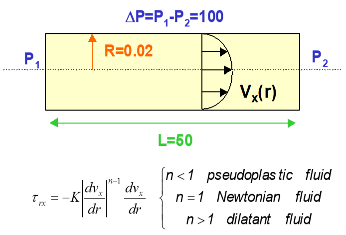
We propose to find the velocity profiles for the laminar flow of Newtonian, power-law and Carreau fluids in a pipe, shown in below.
We use the following values for the pressure difference [Laplacian]P, the exponent n, the Newtonian fluid viscosity η, the consistency index k,
the infinite-shear viscosity, the zero-shear viscosity , the relaxation parameter λ, the pipe length L, and radius R:
[Laplacian]P =100; L = 50; and R = 0.02
Newtonian fluid:
Dilatant fluid: and
Pseudo-plastic fluid: and
Carreau fluid:, , =1.72×, and =0
Reference:
[1] H . Binous, Introducing non-Newtonian fluid mechanics computations with Mathematica® in the undergraduate curriculum, Chemical Engineering Education, 41 (1), pp . 59 - 64, 2007.
[2] J. O. Wilkes, Fluid Mechanics for Chemical Engineers, Upper Saddle River, NJ: Prentice Hall, 1999.
We use the following values for the pressure difference [Laplacian]P, the exponent n, the Newtonian fluid viscosity η, the consistency index k,
the infinite-shear viscosity
η
∞
η
0
[Laplacian]P =100; L = 50; and R = 0.02
Newtonian fluid:
η=8.9×
-4
10
Dilatant fluid:
n=3.39
κ=
-6
10
Pseudo-plastic fluid:
n=0.4
κ=5×
-3
10
Carreau fluid:
n=0.5
λ=0.2
η
0
-3
10
η
∞
Reference:
[1] H . Binous, Introducing non-Newtonian fluid mechanics computations with Mathematica® in the undergraduate curriculum, Chemical Engineering Education, 41 (1), pp . 59 - 64, 2007.
[2] J. O. Wilkes, Fluid Mechanics for Chemical Engineers, Upper Saddle River, NJ: Prentice Hall, 1999.
Acknowledgement :
Since in this laminar flow problem we have split boundary conditions. Problem’s resolution is based on the Shooting Method developed in Mathematica by Professor Brian Higgins (University of California, Davis).
Since in this laminar flow problem we have split boundary conditions. Problem’s resolution is based on the Shooting Method developed in Mathematica by Professor Brian Higgins (University of California, Davis).
Flow of dilatant, pseudoplastic, Carreau and Newtonian fluids in a horizontal pipe.
Flow of dilatant, pseudoplastic, Carreau and Newtonian fluids in a horizontal pipe.
Analytical Solution=1-
v
z
n
n+1
1
n
ΔP
2KL
n+1
n
R
n+1
n
r
R
In[]:=
v
analytical
In[]:=
v
analytical
Out[]=
-1/n
2
1+n
n
r
R
1+n
n
R
1
n
ΔP
KL
1+n
Dilatant Fluid
In[]:=
K=110^-6;n=3.39;ΔP=100;L=50;R=0.02;
In[]:=
system[Ω_]={D[r[r],{r,1}]ΔP/Lr,D[[r],{r,1}]If[[r]≥0,-([r]/K)^(1/n),(-[r]/K)^(1/n)],[10^-5]0,[10^-5]Ω};myODEsoln[Ω_]:=NDSolve[system[Ω],{,},{r,10^-5,R}]yend[Ω_?NumericQ]:=Flatten[([r]/.myODEsoln[Ω])/.rR]bc=FindRoot[yend[Ω]0,{Ω,0,0.5}][[1,2]];
τ
rx
v
x
τ
rx
τ
rx
τ
rx
τ
rx
v
x
v
x
τ
rx
v
x
In[]:=
sol1=myODEsoln[bc]
Out[]=
InterpolatingFunction,InterpolatingFunction
v
x


τ
rx

In[]:=
plt1=Plot[[r]/.sol1,{r,0.00001,R},PlotStyle{Thick,Darker@Green},Frame->True,AspectRatio->1,FrameLabel->{Style["position",14],Style["velocity",14]},GridLines->Automatic,ImageSize->350{1,1}]
v
x
Out[]=
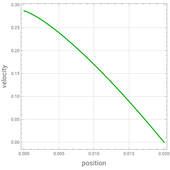
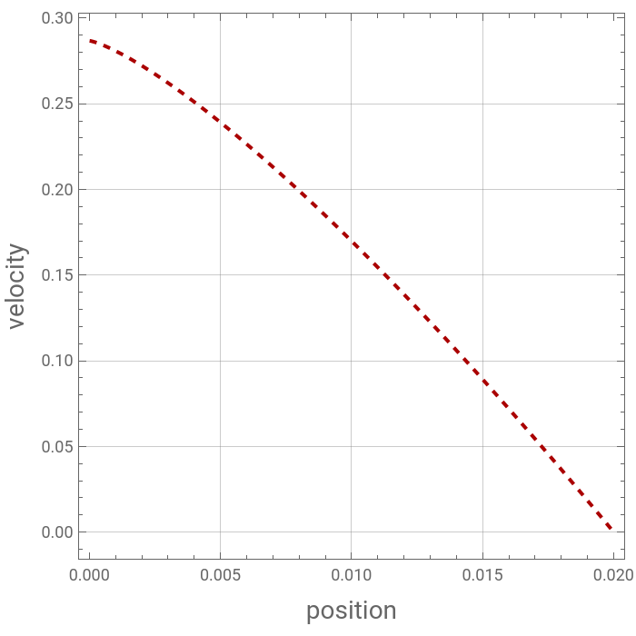
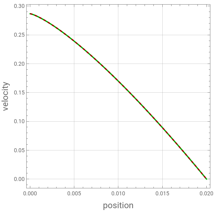
Comparing numerical result (solid line) with analytical solution (dashed curve) for dilatant fluid
In[]:=
plt2=Plot[[r],{r,0.00001,R},PlotStyle{Thick,Darker@Red,Dashed},Frame->True,AspectRatio->1,FrameLabel->{Style["position",14],Style["velocity",14]},GridLines->Automatic,ImageSize->350{1,1}]
v
analytical
Out[]=
In[]:=
Show[plt1,plt2]
Out[]=
Pseudoplastic Fluid
In[]:=
K=510^-3;n=0.4;ΔP=100;L=50;R=0.02;
In[]:=
system[Ω_]={D[r[r],{r,1}]ΔP/Lr,D[[r],{r,1}]If[[r]≥0,-([r]/K)^(1/n),(-[r]/K)^(1/n)],[10^-5]0,[10^-5]Ω};myODEsoln[Ω_]:=NDSolve[system[Ω],{,},{r,10^-5,R}]yend[Ω_?NumericQ]:=Flatten[([r]/.myODEsoln[Ω])/.rR]bc=FindRoot[yend[Ω]0,{Ω,0,0.5}][[1,2]];
τ
rx
v
x
τ
rx
τ
rx
τ
rx
τ
rx
v
x
v
x
τ
rx
v
x
In[]:=
sol2=myODEsoln[bc]
Out[]=
InterpolatingFunction,InterpolatingFunction
v
x

τ
rx

In[]:=
plt3=Plot[[r]/.sol2,{r,0.00001,R},PlotStyle{Thick,Darker@Blue},Frame->True,AspectRatio->1,FrameLabel->{Style["position",14],Style["velocity",14]},GridLines->Automatic,ImageSize->350{1,1}]
v
x
Out[]=
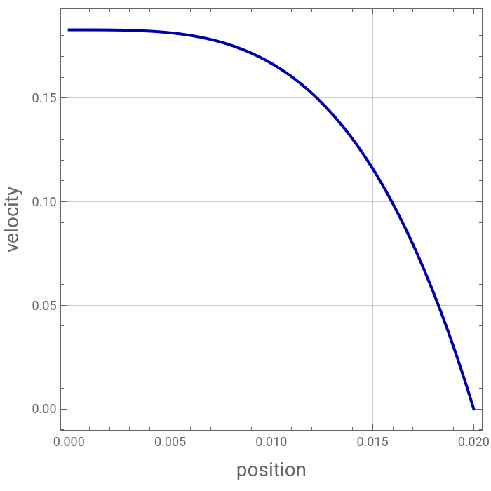
Newtonian Fluid
Comparing numerical result (solid line) with analytical solution (dashed curve) for Newtonian fluid
Comparing velocity profiles obtained for the four fluids: dilatant, pseudoplastic, Carreau and Newtonian.
These profiles are obtained under equal volumetric flow conditions.
The velocity near the wall is higher for Carreau and pseudo-plastic fluids than for Newtonian and dilatant fluids. This results in higher heat transfer rates due to a higher convection.
These profiles are obtained under equal volumetric flow conditions.
The velocity near the wall is higher for Carreau and pseudo-plastic fluids than for Newtonian and dilatant fluids. This results in higher heat transfer rates due to a higher convection.