Overview: Gauge Theories and Symmetries
Overview: Gauge Theories and Symmetries
In physics, the notion of symmetry is a very powerful tool in theoretical physics. We know from Noether theorem that every differentiable symmetry of the action of a physical system has a corresponding conservation law in the form of a conserve current. In other words, if the action of a theory is invariant under the action of some Lie group then we have a corresponding conserved current. In general the potential of a system can be a function of position and time but if we consider theories whose potentials are functions of radial distance |, such as Newtonian gravity and classical electrodynamics where the potential only depends on the radial distance between particles, then the group that keeps the Euclidean inner product invariant known as the special orthogonal group, denoted SO(3), can be considered a symmetry of this system which means that this physical system is globally invariant under the action of SO(3) which via Noether’s theorem implies that there is conserved current, in this case three currents which correspond to the conservation of the three components of angular momentum. Therefore we can talk about invariant quantities within a theory as corresponding to invariance under the action of some continuous Lie group.
Modern colliders, such as the Large Hadron Collider and Relativistic Heavy Ion Collider, provide the context for studying fundamental physics using gauge theories to model the fundamental particles and forces of nature and provides a tool to study the early stages of the universe microseconds before the Big Bang which are beyond the reach of astronomy. These continues symmetries play a critical role along with more mathematically rich symmetries known as local gauge transformations. These symmetries require that physics be invariant under transformations of local “gauge” degrees of freedom, which occur independently at each point in spacetime. The Standard Model of particle physics which is responsible for describing three of the fundamental forces of nature and have been modelled with incredible precision by gauge theories, where the local degrees of freedom are represented by certain well-known Lie groups such as SU(2) and SU(3).
The main obstacle facing theoretical physics is the lack of a unified theory of everything that encompasses gravity, described by the theory of general relativity, and the other 3 fundamental forces described by the Standard Model, many physicists have come to suggested that the continuous nature of spacetime is an approximation which breaks down at the Planck scale. If one adopts this notion that a unified theory of fundamental physics a so called quantum theory of gravity must describe dynamics with some discretized model, which in some continuum limit reproduces both the Standard Model of particle physics and general relativity [1]. This has relevance in the context of the Wolfram models whose are using a discrete constructivist approach to theoretical physics, a new and novel approach to fundamental physics. With this motivation in mind the aim of this project is to construct discrete approximations to continuous gauge filed theories, particularly those studies in high energy physics.
The main goal of this project is to construct and study discrete fibre bundles corresponding to gauge field theories and see how these discrete spaces relate to the Wolfram Model (WM), motivated by the hypergraph-replacement models for fundamental physics proposed in [2]. This project is particularly interested in how one my approximate continuous local gauge symmetries with discrete symmetries corresponding to discrete groups subgroups of Lie groups which can be represented by undirected graphs, namely the Cayley graph of the discrete group. We use the mathematical machinery of differential geometry namely fibre bundles to build an intuition for the characteristics of gauge theories within the context of the Wolfram Model. The main piece of machinery developed in this project is a function that can construct a undirected graph that can be interpreted as a discrete fibre bundle with this tool several investigations were considered, one idea was to demonstrate familiar physical features of the resultant discrete fibre bundle graphs for U(1) electromagnetism on as well as on the torus. This involves defining the discrete analogue of a Wilson loop, while gauge theories built upon discrete networks are well-studied in lattice gauge theory the main different between lattice gauge theory and the theories considered here is that the underlying gauge group in lattice gauge theory is continuous whereas in Wolfram Models we will be approximating these gauge groups with discrete subgroups groups leading to entirely discrete models. Therefore we are attempting to model the world with a discrete universe, where the only meaningful quantities are counts of network connections, where we hypothesise that in the continuum limit the model is able to describe the complexities of the Standard Model. This then leads to the discussion of dynamics on these fibre bundles with the intention of relating these dynamics to re-write rules within the framework of Wolfram Models. The final exploration involves constructing fibre bundles whose base space corresponds to a hyper-graph produced by some re-write rule in the Wolfram Model, with the optimistic goal that one could relate gauge symmetries to re-write rules and the Wolfram Model.
|
r
Modern colliders, such as the Large Hadron Collider and Relativistic Heavy Ion Collider, provide the context for studying fundamental physics using gauge theories to model the fundamental particles and forces of nature and provides a tool to study the early stages of the universe microseconds before the Big Bang which are beyond the reach of astronomy. These continues symmetries play a critical role along with more mathematically rich symmetries known as local gauge transformations. These symmetries require that physics be invariant under transformations of local “gauge” degrees of freedom, which occur independently at each point in spacetime. The Standard Model of particle physics which is responsible for describing three of the fundamental forces of nature and have been modelled with incredible precision by gauge theories, where the local degrees of freedom are represented by certain well-known Lie groups such as SU(2) and SU(3).
The main obstacle facing theoretical physics is the lack of a unified theory of everything that encompasses gravity, described by the theory of general relativity, and the other 3 fundamental forces described by the Standard Model, many physicists have come to suggested that the continuous nature of spacetime is an approximation which breaks down at the Planck scale. If one adopts this notion that a unified theory of fundamental physics a so called quantum theory of gravity must describe dynamics with some discretized model, which in some continuum limit reproduces both the Standard Model of particle physics and general relativity [1]. This has relevance in the context of the Wolfram models whose are using a discrete constructivist approach to theoretical physics, a new and novel approach to fundamental physics. With this motivation in mind the aim of this project is to construct discrete approximations to continuous gauge filed theories, particularly those studies in high energy physics.
The main goal of this project is to construct and study discrete fibre bundles corresponding to gauge field theories and see how these discrete spaces relate to the Wolfram Model (WM), motivated by the hypergraph-replacement models for fundamental physics proposed in [2]. This project is particularly interested in how one my approximate continuous local gauge symmetries with discrete symmetries corresponding to discrete groups subgroups of Lie groups which can be represented by undirected graphs, namely the Cayley graph of the discrete group. We use the mathematical machinery of differential geometry namely fibre bundles to build an intuition for the characteristics of gauge theories within the context of the Wolfram Model. The main piece of machinery developed in this project is a function that can construct a undirected graph that can be interpreted as a discrete fibre bundle with this tool several investigations were considered, one idea was to demonstrate familiar physical features of the resultant discrete fibre bundle graphs for U(1) electromagnetism on
3
Literature Review:
Literature Review:
Differential Geometry and Fibre Bundles
Differential Geometry and Fibre Bundles
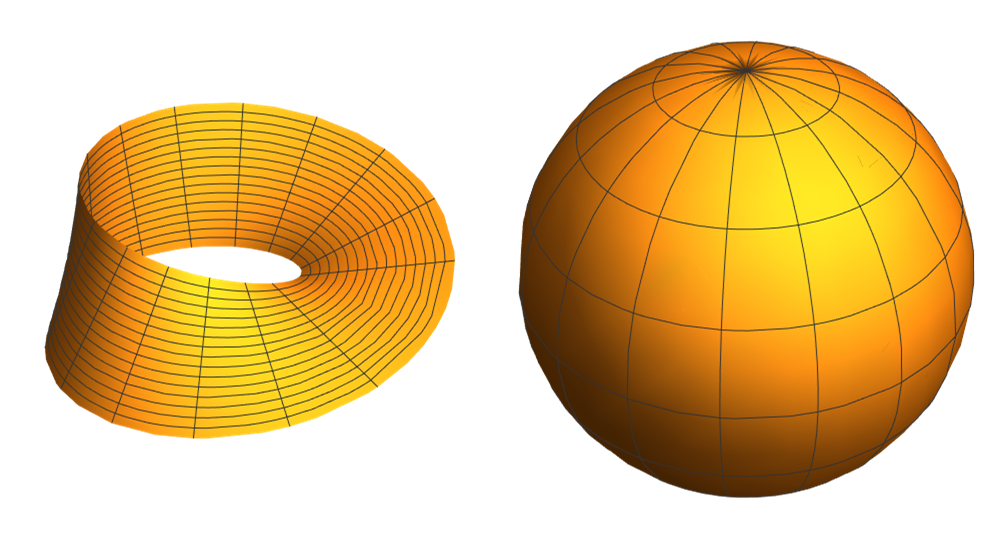
In conventional theoretical physics there is normally a notion of a space where particle can live and interact and all prediction of the theory follow. To formalise this notion of space, one introduces the concept of a manifold which is a generalisation of Euclidean space. A manifold, M is a topological space that locally resembles Euclidean space at each point, this is known as the base space. More precisely, an n-dimensional manifold M is a topological space with the property that each point x ∈ M has a neighborhood that is homeomorphic to an open subset of . One can then define the tangent space at each point x ∈ M which is a n-dimensional real vector space and physical corresponds to the tangents to all the curves that pass through x ∈ M. If one replaces the tangent space at each point x ∈ M with some abstract vector space V, know as a fibre and the collection of all fibres is know as the fibre space denoted F. The fibre bundle is then defined as a topological space E which is locally equivalent to the product M x F of a base space and fibre space, but which globally need not be a trivial product. If this abstract vector space V is replaced with a gauge group G then the resulting fibre bundle is known as a G-principal fibre bundle and the fibres are given by orbits of the gauge group G. A famous non-trivial example of a fibre bundle is the Möbius strip, which may be constructed by inserting the interval [0,1]⊂ along each point on the circle -- locally the Möbius strip is indistinguishable from a cylinder but has a global topological structure that is distinct.
n
T
x
T
x
1
S
Examples of potential base spaces for continuous fibre bundles: The Möbius strip which is the simplest example of a non-trivial fibre bundle and 2-Sphere which will act as the base space to the Hopf fibre bundle discussed in the next section, both plots were generated with ParametricPlot3D.
In[]:=
GraphicsRow[{ParametricPlot3D[{(1+(v/2)Cos[u/2])Cos[u],(1+(v/2)Cos[u/2])Sin[u],(v/2)Sin[u/2]},{u,0,2Pi},{v,-1,1},Boxed->False,Axes->False],ParametricPlot3D[{Cos[u]Sin[v],Sin[u]Sin[v],Cos[v]},{u,0,2Pi},{v,-Pi,Pi},Boxed->False,Axes->False]}]
Out[]=
One then defines a continuous surjective map, π : E ↦ M, which in open subsets of E behaves just like a projection from corresponding regions of M × F to M. The map π is called the projection of the bundle and is regarded as part of the structure of the bundle. The space
E is known as the total space of the fiber bundle, M as the base manifold and F the fiber, this is known as a fibration of the fibre bundle E. The inverse of this map π is a map ϕ: M ↦ E which is a continuous map and are known as sections and this maps continuous paths in the base space to continuous paths in the fibre bundle. If a given fibre bundle has a global section we call that fibre bundle a trivial bundle. The obstruction to the existence of a section can often be measured by a cohomology class, which leads to the theory of characteristic classes in algebraic topology, the main mathematical underpinning of this project comes from [3] where these homotopy classes of closed loops in the bundle relate to the curvature of the bundle. The final object one needs to construct a fibre bundle is the connection. Since each point in the base space M has a unique fibre if one wants to compare elements of nearby fibres we must identify a map between them, this leads to the notion of parallel transport which describes how tangent vectors transform as they move along paths in curved space time. In gauge theory the choice of gauge leads to the notion of curvature and defines the gauge field configuration. We may then think of a connection as a rule which for any path in the base space M returns a path through the bundle.
Before we begin to investigate the discrete approximations of principal fibre bundles lets consider some standard well understood continuous case, namely the Hopf fibre bundle.
Hopf Fibre Bundle and Hopf Fibration
Hopf Fibre Bundle and Hopf Fibration
The Hopf fibration, named after Heinz Hopf who studied it in a 1931 paper [4], is an important object in mathematics and physics. It was a landmark discovery in topology and is a fundamental object in the theory of Lie groups. The Hopf fibration has a wide variety of physical applications including magnetic monopoles, rigid body mechanics and quantum information theory. The Hopf fibration is the mapping → defined by
h:
3
S
2
S
In[]:=
HopfFibration=#/.{a_,b_,c_,d_}:>{a^2+b^2-c^2-d^2,2(ad+bc),2(bd-ac)}&;{,,,}//HopfFibration
a
1
a
2
a
3
a
4
Out[]=
+--,2(+),2(-+)
2
a
1
2
a
2
2
a
3
2
a
4
a
2
a
3
a
1
a
4
a
1
a
3
a
2
a
4
where istheunit sphere in .One finds that circles in are mapped to points in , leading to the natural geometric interpretation of the fibre bundle where each point in the base space is mapped onto fibre which in this case is a circle on the surface of .
n
S
n+1
3
S
2
S
3
S
In[]:=
{Cos[x],Sin[x],0,0}//HopfFibration//Simplify
Out[]=
{1,0,0}
The Hopf fibre bundle is an example of a non-trivial fibre bundle with as the base manifold and the gauge group U(1) ≅ are the fibres, therefore the map h is a fibration of the Hopf fibre bundle. The work in Hopf’s paper [4] was an early achievement in the modern subject of homotopy theory. In simple terms, homotopy seeks to understand those properties of a space that are not altered by continuous deformations. The Hopf fibre bundle has an intimate relationship with rotation in and the quaternions. A point P = (x, y, z) on the base manifold can be represented by a unit pure quaternion P = x + y + z then for any quaternion r = a + b + c + d we can define a rotation ∈ . Lets now chose P = (1, 0, 0) then the Hopf fibration h defined above can be written in terms of quaternions as follows,
2
S
1
S
3
2
S
R
r
3
In[]:=
ResourceFunction["Quaternion"][a,b,c,d]**ResourceFunction["Quaternion"][0,1,0,0]//#**ResourceFunction["Quaternion"][a,-b,-c,-d]&
Out[]=
For any point P in (represented as a pure quaternion), the preimage set (P) is a circle in and is preformed using the function HopfFibre defined below. We will also refer to the preimage set (P) as the fiber of the Hopf map over P and an expression for is given by [4]
2
S
-1
h
3
S
-1
h
-1
h
In[]:=
HopfFibre[{-1,0,0}]:=ResourceFunction["Quaternion"][0,0,0,1]//#**ResourceFunction["Quaternion"][Cos[t],Sin[t],0,0]&;HopfFibre[{p1_,p2_,p3_}]:=ResourceFunction["Quaternion"][0,1+p1,p2,p3]//1/Sqrt[2(1+p1)]*#&//#**ResourceFunction["Quaternion"][Cos[t],Sin[t],0,0]&
and notice again that points on are mapped onto circles on whose points are represented by unit quaternions, this map need not be unique.
2
S
3
S
In[]:=
{1,0,0}//HopfFibre
Out[]=
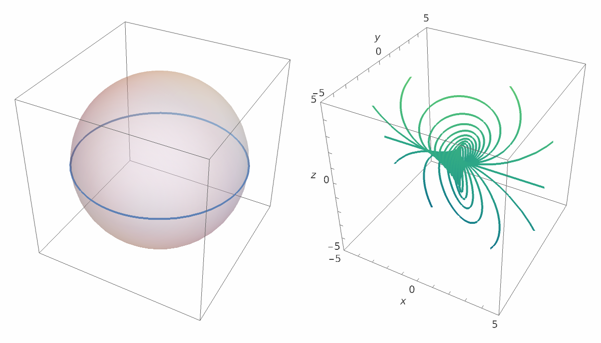
The stereographic projection generalizes to all dimensions, and in particular, it provides a projection map \{1,0,0,0} → . The real power of stereographic projection is that it allows us to see all of the 3-sphere (except one point) in familiar 3-space. This is remarkable because is a curved object that resides in 4-space. Therefore it in not possible to visualise sections in the Hopf bundle. Each point in the base manifold is mapped onto a circle on which via the stereographic projection is mapped onto a circle in , this is due to the fact that the stereographic projection preserves circles. So in the images below we see that as one travels along a circle in the base space one traces out a surface in comprised of a circle for each point along the path in the base space. The explicit expression for the stereographic projection f: \{1,0,0,0} → is given byf(w, x, y, x) = (x,y,z).
3
S
3
3
S
2
S
3
S
3
2
S
4
3
S
3
1
1-w
In[]:=
StereographicProjection[a_]:=1/(1-a[[1]]){a[[2]],a[[3]],a[[4]]}
A graphical representation of the Hopf fibre bundle, the base space is with a U(1) fibre structure. Each point in the base space has a corresponding fibre which is visualised by using the stereographic projection to map circle on into circles in . A function that preforms the projection is defined below, then each point in the base space is mapped into a fibre by using HopfFibre then is projected into using StereographicProjections, these are visualised using ParametricPlot3D.
2
S
3
S
3
3
In[]:=
HopfBase1=Show[Graphics3D[{Opacity[0.3],Sphere[{0,0,0},1]}],ParametricPlot3D[{Cos[t],Sin[t],0},{t,0,2Pi},ColorFunction->Hue[y]]];HopfBase2=Show[Graphics3D[{Opacity[0.3],Sphere[{0,0,0},1]}],ParametricPlot3D[{Cos[t]Sin[Pi/4],Sin[t]Sin[Pi/4],Cos[Pi/4]},{t,0,2Pi},ColorFunction->Hue[y]]];HopfFibres1=Table[{Cos[t],Sin[t],0},{t,0,2Pi,Pi/10}]//Simplify//HopfFibre/@#&//StereographicProjection/@#&//ParametricPlot3D[#,{t,0,2Pi},ColorFunction->"BlueGreenYellow",PlotRange->{{-5,5},{-5,5},{-5,5}},Axes->True,AxesLabel->{x,y,z}]&;HopfFibres2=Table[{Cos[t]Sin[Pi/4],Sin[t]Sin[Pi/4],Cos[Pi/4]},{t,0,2Pi,Pi/10}]//Simplify//HopfFibre/@#&//StereographicProjection/@#&//ParametricPlot3D[#,{t,0,2Pi},ColorFunction->"BlueGreenYellow",PlotRange->{{-5,5},{-5,5},{-5,5}},Axes->True,AxesLabel->{x,y,z}]&;GraphicsRow[{HopfBase1,HopfFibres1}]
Out[]=
Discrete Gauge Field Theory
Discrete Gauge Field Theory
Constructing a General Discrete Fibre Bundle
Constructing a General Discrete Fibre Bundle
Now that we have considered a standard example of a non-trivial continuous fibre bundle and gained an intuition for the basic geometric structure of fibre bundles. We can now begin to think about fibre bundles in discrete geometries. When one considers the discretization of fibre bundles the notion of base space will in general be some undirected graph which can be interpreted as a discrete approximation to some continuous base manifold. The gauge group G whose orbit comprise the fibres of the bundle will be replaced with a discrete objects that can be represented by undirected graphs. We approximate a continuous Lie group with a discrete subgroups. By Cayley’s theorem, any finite (sub-)group may be represented as a permutation group over its set of elements, therefore any discrete subgroup of a Lie group that one wants to use to approximate continuous Lie group is isomorphic to some subset of the permutation group. This finite permutation group has a graph representation given by the Cayley graph of the permutation group which we will denote for fibre graph.
Now that we have established a notion of base space and fibres for discrete fibre bundles, the final piece of information one needs is the connection information. When we move to this discrete structure, any path through the base space graph consists of a sequence of edges between vertices. In order to define a connection in this discrete setting, we assume that the entire bundle must also be described by a graph ,where connections lift edges in the base space graph to edges in the bundle graph via some edge lifting map C: ] ↦ ] i.e. the connection determines which edge one must travel along in the bundle when travelling between neighbouring fibres that correspond to neighbouring points in the base graph. We will see that this identification has consequences for the connectivity of and its physical interpretation. Now the final step is to define parallel transport on these bundles, in the case of lattice gauge theory the parallel transport operators which encode how the gauge group action is communicated between neighbouring lattice sites. In the case of lattice gauge theory these operators take values in the Lie algebra of the gauge group G. However in the discrete setting there is no clear way of defining a Lie algebra so these parallel transport operators take values in the from the discrete gauge group, now denoted G. Therefore by assigning an element of G to each edge in the base space graph we fully specify the gauge configuration of the bundle.
Therefore when constructing these G-bundle graphs we begin by inserting a copy of the minimal subgraph of the gauge group G at each vertex in the base graph. Function are defined here that takes in a base space graph, the generators of a finite permutation group and connection information (an associative array where each edge in the base space graph is assigned a gauge group element) and constructs the corresponding G-bundle graph, this function is called CreateFibreBundleGraph. The function CreateFibreBundleGraph was created inorder to generalise the work done in [1] to allow one to construct a discrete principal fibre bundle that corresponds to a theory with an arbitrary base space, discrete gauge group and connection. This function is used to verify the results from [1] and expand the exploration to study dynamics on these fibre bundles. An additional application of this function would be to use the output fibre bundles to compare to (hyper-)graphs produced by the Wolfram model and potentially one could identify which re-write rule producers certain discrete symmetries.
Below we consider a few basic examples of discrete fibre bundles
G
M
G
F
Now that we have established a notion of base space
G
M
G
F
G
M
G
E
G
M
G
E
E[
G
M
E[
G
E
G
E
G
M
Therefore when constructing these G-bundle graphs we begin by inserting a copy of the minimal subgraph of the gauge group G at each vertex in the base graph
G
M
Below we consider a few basic examples of discrete fibre bundles
Example 1: 3 × U(1)
Example 1: × U(1)
3
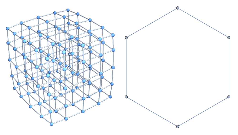
A more interesting example and one that we will return to later is the × U(1) bundle, this fibre bundle would be a discrete approximation of a gauge theory that would resemble U(1)-electrodynamics. This bundle will be of interest in the next section where we will attempt to define the discrete analogue of a Wilson loop where we will attempt to study the magnetic monopole distribution of this bundle for both a flat and non-flat connection. The base space and fibre are shown below.
3
In[]:=
base2=GridGraph[{5,5,5}];group2=CyclicGroup[6]//GroupGenerators;conn2=Cycles[{{}}];GraphicsRow[{base2//GraphPlot3D,group2//PermutationGroup//CayleyGraph//UndirectedGraph}]
Out[]=
In[]:=
bundle2=CreateFibreBundleGraph[base2,group2,conn2];
The function CreateFibreBundleGraph creates the corresponding bundle graph from the 3-D lattice and where each colour corresponds to a fibre at a given point. Notice that this is a trivial bundle since there exists a global section, a section that travels through every fibre. The base space consist of 2550 edges and there are 6 elements in the gauge group, therefore for each edge in the base space there are six choices of connection leading to ~ 2 choices of dynamical gauge configuration and is the discrete analogue of gauge freedom in discrete gauge field theory.
C
6
2550
6
1985
10
The final example of an output from CreateFibreBundleGraph the example of the torus which is a U(1)-bundle on a circle. The base space and fibre graph are given by;
This then creates a torus that is isomorphic to the built-in TorusGraph native to Mathematica.
Therefore as one travels through the bundle it is possible to examine the additivity of Wilson loops by summing up these phases which correspond to flux integrals through surfaces in the bundle. Now since we have selected a connection for each edge in the base space this sum will be possible, we are now faced with the problem of calculating closed loops in the base space, luckily Mathematica has a function for this. We may think of any Wilson loop as indicating the magnetic flux across its (oriented) subtended surface [6]. The 1st Chern number in this setting quantifies the total emanating flux from a volume. So in principal one would calculate the value of these Wilson loops by finding a closed path through the base and summing up the phases of all the connections along the loop, this can be interpreted as the discrete analogue of a flux integral, therefore non-zero values correspond to a non-zero magnetic flux through a hyper surface in the fibre bundle which can be interpreted as a existence of a Dirac magnetic monopole at that point in the base space. To find closed paths through the base space, this process depends on the particular choice of base space. This interpretation of phase is only natural and unambiguous is gauge groups that are discrete approximations of U(1), much more work needs to be done to understand Chern numbers and there link to physical quantities in discrete gauge field theories.
The Flat connection
The Flat connection
Then using a function I created called MonopoleDistribution which takes in the base space, gauge group and connection information as input and returns the magnetic charge at each vertex in the base space. The magnetic flux at a vertex v is calculated by finding the shortest closed loop that includes v and then summing over the phases of all the gauge group elements that represent the connections along that path. This procedure allows one to calculate the magnetic charge at each point in the base space. As mentioned above, we expect the monopole distribution to be zero for any choice of global connection which is indeed the case. In fact the distribution is zero for an choice of global connection and is a result of the topological triviality of the bundle.
Random Connection
Random Connection
Now if we give our bundle a random gauge configuration, we expect there to be a non-trivial distribution of magnetic charge i.e. we assign a random gauge group element to each edge in the base graph. However, there still remains ambiguity regarding total flux: it is possible [6] for the net flux out of a volume to take on non-zero values which are integer multiples of 2π. These configurations may be interpreted as magnetic monopoles, which are not forbidden at the lattice scale. We observe that for a random gauge configuration, there is a non-trivial distribution of magnetic charge. This distribution appears to be heavily biased towards positive charge -- however this is only due to the choice of π in the ambiguous phase assignment for the square root of the identity. In the continuum limit to U(1), the measure of this particular group element drops to zero, and this asymmetry vanishes.
The it is possible to observe a non-zero distribution of magnetic monopoles, the figures below show the monopole distribution of our fibre bundle where the red colours represents positive charge and the blue colours represent negative charge. Note that the distribution is heavily biased towards positive charge which is due to the choice of π over -π in the phase assignment.
U(1)-Electrodynamics on Torus
U(1)-Electrodynamics on Torus
This leads to a bundle graph that looks like
With a random gauge configuration we have the following monopole distribution of the torus.
Introducing Dynamics & Wolfram Model
Introducing Dynamics & Wolfram Model
Now that all the tools have been put in place it is now possible to start introducing dynamics to the model;
One idea is to have fibre bundles with a global flat connection and then one can introduce a defect to the lattice that can correspond to one of the connections in the bundle being non-trivial. The non-zero phase of this connection will result in a non-trivial distribution of Dirac monopoles whose sign will be determined by the sign of the phase of the artificially introduced connection. One could then introduce two such connections, where one has a positive phase and other having a negative phase leading to a distribution of charges that is overall neutral, then one could let this defect travel through the bundle is some causal way i.e. the defect can travel to edges in the base space that share a vertex with the edge corresponding to the defect. In this was we have a mechanism for monopoles to move along a path in the base space, this is just a toy model and far more work can go into exploring dynamics that are more realistic.
Another interesting idea is to construct fibre bundles whose base spaces are (hyper-)graphs that are produced by using re-write rules within the context of the Wolfram Model. This could help researcher gain insight into the Wolfram Model and as a long term goal one might be able to classify re-write rules and identify if particular collections of re-write rules lead to topological structures encountered in a more traditional theoretical physics settings. If the Wolfram Model is indeed a model of every universe then one could naively speculate that there is some subset of re-write rules that manifest physically realizable theories, this bring us back to the issue that more work needs to go into studying discrete gauge field theories and their links to physically measurable/observable quantities. This would require one to build on the work laid out in [3] to develop computational machinery to do calculations of measurable quantities on discrete fibre bundles.
Both these ideas are briefly explored below.
Incorporating Re-write Rules: Dipole Random Walks
Incorporating Re-write Rules: Dipole Random Walks
Whose fibre bundle graph is given by
The connection structure of the bundle is chosen to be the global flat connection, then as prescribed above we introduce two non-flat connections (connections with non-zero phase) to the lattice. The non-zero phase of this connection will result in a non-trivial distribution of Dirac monopoles whose signs will be determined by the signs of the phase of the two artificially introduced connections where the one connection has a positive phase and other connection has a negative phase leading to a distribution of charges that is overall neutral and approximates a magnetic dipole Then one could let this defect travel through the bundle is some confluent way. This process is visualised below where positive charge in the base space are represent by red squares and and negative charges by blue squares. The notion of causality is introduced by only allowing the non-flat connection to move to a edge that is neighbouring the edge that currently has the non-flat connection. The charges are given initial edges that are in opposite corners of the base space and the simulation runs for a fixed number of times steps (re-writes).
There are a few interesting things to note here. Firstly the re-write rules do not conserve the charge on the bundle, this is due to the fact that there is no unique way to define a Wilson loop in this context and there is some ambiguity as to how one chose the Wilson loops. The form of the charge distribution is therefore dependant on the choice of path for the Wilson loop. Secondly, these charges follow no deterministic path since they have been chose to follow random paths through the base space. It is possible for two oppositely charged monopoles to annihilate and form a neutrally charges object. Naively one may liken this process to the creation-annihilation of electron-positron pairs in theories that feature in the Standard Model although this situation is far different and involves physical object that have not been observed through experimental techniques.
Bundles on Wolfram Models
Bundles on Wolfram Models
Whose bundle graph with U(1) is given by
Notice that there is now a discrete set of vertices at each point in the base space. This in principal be use to construct a fibre bundle from any given hyper-graph produced by the Wolfram Model and is a step in the right direction to start investigating how gauge theories can be derive through re-write rules in multi-way systems. A initial idea is to create fibre bundle from Wolfram Model hypergraphs with a given discrete symmetry and use a function developed in Jessica Yuan’s project named SpectraGraphDistance to measure the distance between the base space and the fibre. Once could compare the distance between the base graph and bundle graph at each step in the rewrite process. Another interesting option would be to construct fibre bundle from Wolfram hypergraphs and compare this bundle graph to other hyper-graphs and one could see if it is possible to construct multi-way systems that have a definite discrete gauge symmetry.
Conclusion & Outlook
Conclusion & Outlook
The work done in this project builds on the work in [1] and the ability to, in principal, construct any principal fibre bundle for a discrete base space and discrete gauge group. This is a major step in towards generalizing the gauge field theories to discrete fibre bundle in an attempt to connect gauge field theories to discrete model of fundamental physics which involves graphs and hypergraphs. The project has achieved the goal of setting up the machinery to study gauge theories on discrete fibre bundles, we have been able to build up this discrete theory with a few illustrative examples and have been able to arrive at a concrete notion of parallel transport and gauge freedom in these discrete models. This then allowed us to calculate some physically relevant quantities on these discrete spaces although magnetic monopole density is not truly a physically measurable quantity as they have not been observed through experiment. Finally we were able to introduce some form of dynamics to the model by using a modified version of re-writing rules to propagate the magnetic monopoles through the bundle such that the local gauge symmetry is preserved for each time step. The final section attempted to relate the work done in this project to the Wolfram Model, this was done by creating fibre bundles whose bases space were Wolfram Model hypergraphs.
However, this discretization of gauge theories is not without draw backs and the introduction of a discrete gauge group leads to ambiguities which depends on the choice of phase interpretation. The introduction of a discrete base space leads to an ambiguous definition of Wilson loops. Even in the simplest cases we have observed anomalies which depend upon our choice of phase interpretation of the discrete gauge group. The are many paths for future research, one path would be to fully explore the dynamics of the model. In this way we will gain a clearer understanding of how evolution must proceed in order to respect both the global and local gauge symmetry of the bundle, this may lead to insight on how re-write rules relate to symmetries in physics. Another avenue for future research would be to build on the work developed in [3] and extend the study to non-Abelian gauge groups including SU(2) and SU(3), which will allow us to calculate instanton numbers on these bundles and start to work with non-Abelian gauge theories on discrete space-time. Finally I would like to thank the WSS 2021 for a great experience.
However, this discretization of gauge theories is not without draw backs and the introduction of a discrete gauge group leads to ambiguities which depends on the choice of phase interpretation. The introduction of a discrete base space leads to an ambiguous definition of Wilson loops. Even in the simplest cases we have observed anomalies which depend upon our choice of phase interpretation of the discrete gauge group. The are many paths for future research, one path would be to fully explore the dynamics of the model. In this way we will gain a clearer understanding of how evolution must proceed in order to respect both the global and local gauge symmetry of the bundle, this may lead to insight on how re-write rules relate to symmetries in physics. Another avenue for future research would be to build on the work developed in [3] and extend the study to non-Abelian gauge groups including SU(2) and SU(3), which will allow us to calculate instanton numbers on these bundles and start to work with non-Abelian gauge theories on discrete space-time. Finally I would like to thank the WSS 2021 for a great experience.
Acknowledgment
Acknowledgment
Mentor: Jon Lederman
Firstly I would like to thank everyone involved in the Wolfram Summer School (WSS), this has been a truly unforgettable experience. I would then like to thank my mentor Jon Lederman for guiding me through the summer school and always providing good advice. I also would like to thank Taliesin Beynon helping introduce me to discrete geometry. Thank you to Jonathan Gorard and Xerxes Arsiwalla for assisting in the project selection process and answering my questions during their busy office hours. Additionally I would like to thank Matt Kafka (and Xerxes) for discussing the statistical physics aspects of the Wolfram Model which was very interesting and I hope I will be able to assist with aspect of these statistical physics simulations in the future. Finally a big thank you to Erin Cherry for here support and organisational skill throughout the WSS.
References
References
◼
[1] Graham Van Goffrier, “Full Discretization of Local Gauge Invariance”, University College London (2020): https://community.wolfram.com/groups/-/m/t/2030337
◼
[2] Wolfram Physics Project: Technical Documentation. https://www.wolframphysics.org/technical-introduction/
◼
[3] Manton, N. S. Connections on discrete fibre bundles. Comm. Math. Phys. 113 (1987), no. 2, 341--351. https://projecteuclid.org/euclid.cmp/1104160217
◼
[4] H. Hopf, “Über die Abbildungen der dreidimensionalen Sphare auf die Kugelflache”, Math. Ann. 104 (1931), 637–665
◼
◼
[6] Prouse, N.W. Magnetic Monopoles in Pure Compact Lattice Quantum Electrodynamics. Thesis, Imperial College London. https://www.imperial.ac.uk/media/imperial-college/research-centres-and-groups/theoretical-physics/msc/dissertations/2014/Nicholas-Prouse-Dissertation.pdf