Authors
Authors
Abstract
Abstract
Train and subway systems can be easily modeled as networks, where stations are vertices and connections are edges. In this project, the London Subway system is analyzed using methods from graph theory to understand station importance, network robustness, and underlying community structure. Betweenness centrality is used to identify critical stations that play a key role in routing and navigation, and the effect of station removal on overall network functionality is quantified through changes in average betweenness. Network resilience is further explored by randomly removing nodes and edges and tracking the size of the largest connected component as a function of removal fraction. Finally, multiple community-detection techniques; including modularity-based, spectral, and weighted clustering; are applied to identify sub-networks within the subway system. Together, these analyses show how the London Underground balances efficiency, structural organization and more.
Introduction
Introduction
Transportation networks, such as subway networks, are essential infrastructures where the efficiency and resilience directly affect millions of daily users. Graph theory is a powerful framework for modeling such systems, allowing stations to be represented as vertices, and connections made by tracks as edges. Using this, measures such as centrality, connectivity, and modularity can be used to quantify both local importance and global system behavior.
Selecting Data
Selecting Data
Loading the London Underground (subway network) graph dataset:
In[]:=
london=ResourceData["London Subway Network"];
Making sure the graph runs both ways (like a subway station) and therefore deleting duplicate paths. It should be already clean because it is built-in, but this step is to make sure:
In[]:=
g0=SimpleGraph[UndirectedGraph[london]];
Original Values of Vertex and Edge Counts:
In[]:=
v0=VertexCount[g0]e0=EdgeCount[g0]
Out[]=
353
Out[]=
409
Setting the seed so outputs are more reproducible:
SeedRandom[1234];
Modeling Network Resilience in the Large Scale
Modeling Network Resilience in the Large Scale
In this section, we will be exploring the large-scale resilience of the London Subway Network under random failures. We simulate such failures, like of stations or segments of a subway line, by randomly removing nodes and edges from its graph model. By adjusting the fraction of nodes or edges removed from the graph, we can analyze how the overall connectivity degrades, and therefore receive a metric that may be used to compare network health with other subways. Through the analysis of random trials, we identify characteristic thresholds where the network fragments. The results gathered from the data provide an empirical insight of when the system “falls apart” and allows comparison between node and edge-level failures.
Network resilience can be defined in many ways, depending on the application. In this project, we focus on connectivity resilience: the ability of stations to remain mutually reachable as failures occur.
Specifically, we quantify this by the size of the largest connected component (LCC) during our experiments on the London Underground. The LCC represents the largest subset of stations that are still mutually connected. Its size is the number of nodes in this subset. We normalize its size by the number of stations in the original network, producing a value between 0 and 1. Values near 1 indicate that most of the system remains connected, while values near 0 indicate severe fragmentation.
Therefore, the LCC fraction is the size of the largest connected component of the resulting graph, divided by v0.
Baseline Functions and Definitions
Baseline Functions and Definitions
The “LCC fraction” is the normalized largest connected component size explained above. It is our focused metric for measuring fragmentation severity in our graph.
A function that calculates the LCC size:
In[]:=
LCCSize[g_]:=If[VertexCount[g]==0,0,Max[Length/@ConnectedComponents[g]]];
Let’s take a look at what the LCC is on the unmodified graph:
In[]:=
LCCSize[g0]
Out[]=
353
The graph is fully connected, as the LCC size is the same as the vertex count.
This calculates the size of the LCC fraction of an inputted graph compared to g0:
In[]:=
fractionLCC[g_,v0_:v0]:=(*sizeofLCC/g0size*)N[LCCSize[g]/v0];
Random Node and Edge Removal
Random Node and Edge Removal
We simulate failures by randomly removing either stations (node removal) or track segments (edge removal). Removing a fraction 𝑝 of nodes models scenarios such as station closures or localized outages, while removing edges models track failures or service disruptions between stations. Because individual random deletions can produce noisy results, we repeat each experiment many times and average the resulting LCC fractions. This allows us to observe the typical large scale behavior of the network rather than outcomes driven by pure random chance.
Node (Station) Removal
Node (Station) Removal
This function will output one LCC fraction (as a decimal) after randomly deleting a fraction 𝑝 of the nodes in g0:
randomNodeRemovalFrac[p_]:=Module[{deleteNum=Round[p*v0],deleteList={}},deleteList=RandomSample[VertexList[g0],deleteNum];fractionLCC[VertexDelete[g0,deleteList]]];
Let’s test it. Notice how the size of the LCC fractions will generally decrease as removal fraction 𝑝 increases, which makes intuitive sense.
Outputs a list of LCC fractions for values of 𝑝 from 0.0 to 0.5 in interval of 0.1:
In[]:=
N[Table[randomNodeRemovalFrac[p],{p,0,0.5,0.1}]]
Out[]=
{1.,0.730878,0.473088,0.195467,0.0651558,0.0311615}
Edge (Segment) Removal
Edge (Segment) Removal
This function is similar to the randomNodeRemovalFrac function, except that we delete a certain random amount of edges instead:
In[]:=
randomEdgeRemovalFrac[p_]:=Module[{deleteNum=Round[p*e0],deleteList={}},deleteList=RandomSample[EdgeList[g0],deleteNum];fractionLCC[EdgeDelete[g0,deleteList]]];
Computation
Computation
To study how resilience changes gradually, we evaluate the network over a range of removal fractions 𝑝. For each value of 𝑝, we perform multiple independent trials and compute the average LCC fraction of those trials. The result is a smooth curve that describes how global connectivity degrades as failures accumulate.
For our experiment, we decided to take 𝑝 in intervals of 0.05 (this can be changed; it just takes longer to test and run), which gives us 20 values for 𝑝 from 0.0-0.95 inclusive.
The data range of 𝑝 used for our trials:
In[]:=
dataInterval=Range[0.0,0.95,0.05];
This outputs a single set of trials given a range for 𝑝 and type of removal (node or edge):
singleRun[range_,trialNum_,removalFunc_]:=Table[Mean[Table[removalFunc[p],{trialNum}]],{p,range}]
Testing the single trial function 50 times to create a set of trials for node and edge data:
In[]:=
nodeData:=singleRun[dataInterval,50,randomNodeRemovalFrac];(*Thisisonesetof50trials.Onetrialhas20datapoints*)edgeData:=singleRun[dataInterval,50,randomEdgeRemovalFrac];
Now, we will have a set of trial data so we are able to compare their graphs.
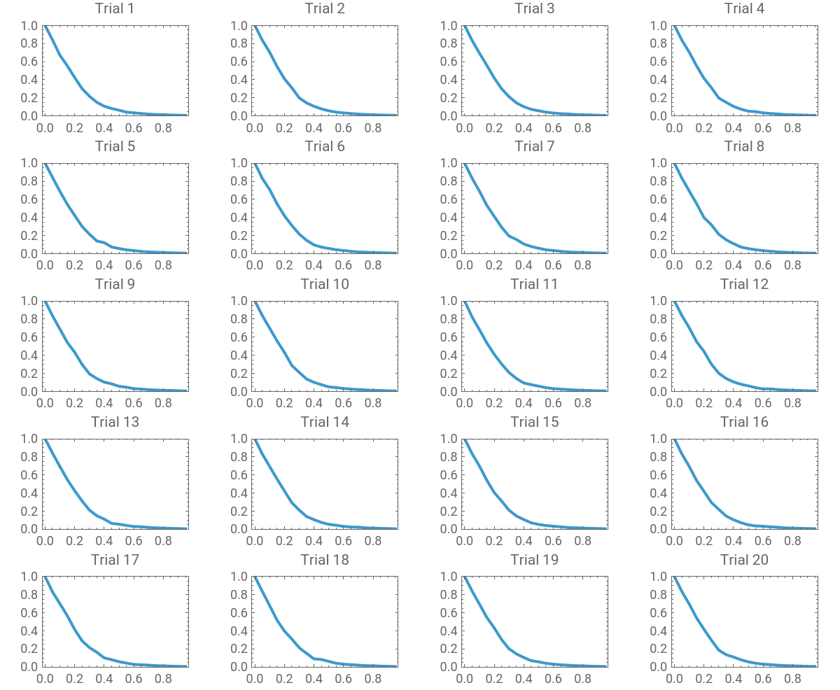
Even when averaged, random processes may still exhibit variability. To quantify how stable the removal fraction pattern is, we generate many independent LCC curves and analyze their spread. This allows us to distinguish consistent structural behavior from randomness, which helps in confirming the accuracy of our results.
This runs 20 sets each of node and edge removal trials:
In[]:=
nodeDataEXP=Table[nodeData,{20}];(*thisis20sets*)edgeDataEXP=Table[edgeData,{20}];(*thisis20setsoftrials*)
This computes the mean of the LCC fractions for each 𝑝 for nodeDataEXP:
In[]:=
nodeDataMean=Mean/@Transpose[nodeDataEXP];(*meansofeachsetoftrials*)edgeDataMean=Mean/@Transpose[edgeDataEXP];(*meansofeachsetoftrials*)
Calculating the standard deviations across edge and node trials:
edgeDataStdev=StandardDeviation/@Transpose[edgeDataEXP](*stdevsofeachsetoftrials*)nodeDataStdev=StandardDeviation/@Transpose[nodeDataEXP](*stdevsofeachsetoftrials*)
The relatively small standard deviation across trials indicates that the observed degradation pattern is a solid and can be used for accurate conclusions on the subway network’s resilience.
Graphs
Graphs
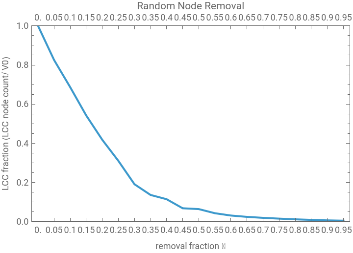
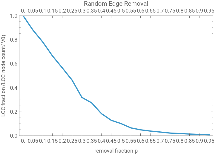
The plots below show how the connectivity of the London Underground changes as a fraction 𝑝 of stations or track segments is removed at random. Each curve represents the largest connected component on the y-axis and the removal fraction on the x-axis.These graphs provide a visual comparison of how node and edge failures degrade global connectivity and lead into the threshold and slope analyses that follow.
This curve represents one set of trials (using our nodeData value), which shows the change in size of its LCC fraction as we increase 𝑝 (the removal fraction). We graphed it here to show an enlarged view of what the graph is meant to look like.
In[]:=
ListLinePlotTranspose[{dataInterval,nodeData}],Frame->True,PlotRange->{0,1},FrameLabel->"removal fraction 𝑝","LCC fraction (LCC node count/ v0)",PlotLabel->"Random Node Removal",FrameTicks->{dataInterval,Automatic}
Out[]=
This curve represents one set of trials (using our edgeData value), which shows the change in size of its LCC fraction as we increase 𝑝 (the removal fraction).
ListLinePlotTranspose[{dataInterval,edgeData}],Frame->True,PlotRange->{0,1},FrameLabel->"removal fraction 𝑝","LCC fraction (LCC node count/ v0)",PlotLabel->"Random Edge Removal",FrameTicks->{dataInterval,Automatic}
Out[]=
Here are graphs of all the sets of trials in nodeDataEXP:
In[]:=
GraphicsGrid[Partition[MapIndexed[ListLinePlot[Transpose[{dataInterval,#1}],Frame->True,PlotRange->{0,1},FrameLabel->None,(*removelabels*)FrameTicks->{Automatic,Automatic},(*keepticks*)PlotLabel->("Trial "<>ToString[#2[[1]]]),ImageSize->600]&,nodeDataEXP],UpTo[4]],Spacings->{1.5,1.5}]
Out[]=
We notice that both graphs give us a curved shape for our LCC fraction, meaning the network does not “fall apart” in a linear fashion.
Analysis and Damage Assessment
Analysis and Damage Assessment
We define the severity of the network fragmentation (how much it “falls apart”) as such:
◼
An LCC fraction of 0.9 or greater means minor fragmentation.
◼
An LCC fraction of 0.7 to 0.9 means moderate fragmentation.
◼
An LCC fraction of 0.5 to 0.7 means severe fragmentation.
◼
An LCC fraction of less than 0.5 means critical damage (and therefore the network has fallen apart).
Note that this is not a standardized, widely used fragmentation guide, as there is numerous different values for determining what counts a graph as “falling apart.”
From here, we will begin to interpret our data and reach conclusions, like about our removal fractions at certain thresholds and steepest parts of the graphs.
First, we will find the critical thresholds, which help us see what removal fraction is corresponding.
This function returns the removal fraction at which the LCC fraction will be below a certain number (input) according to inputted data:
We will now test our criticalThreshold function.
Calculate critical thresholds for 0.9 and 0.65 LCC fraction values, for each set of trials:
Notice how the critical thresholds stay the same for all of these trials. We can quite confidently conclude that the removal fractions will stay near constant across all different trials .
Here’s a list of the key thresholds we will be testing for that correspond to our fragmentation guide. The 0.1 value is there as an extra metric:
Now we will see the removal fractions for each given threshold:
Testing the function:
Sorts the LCC fraction into fragmentation categories:
Combines the removal fraction data we have into a clean table and categorizes the severity of fragmentation at the LCC thresholds:
Slope Calculation and Final Combined Graphs
Slope Calculation and Final Combined Graphs
Beyond fixed thresholds, it is also useful to identify where connectivity collapses most rapidly. We compute the discrete slope of the LCC curve and locate the interval with the steepest decline. This marks a tipping point where a small increase in failures leads to a disproportionately large loss of connectivity.
Here is the code for finding the removal fraction interval in which the slope is the greatest (greatest drop):
Calculating the maximum slopes and the intervals in which they occur, according to the means of node and edge data:
This data tells us that between 𝑝 values of 0 and 0.05 (0% and 5%), the LCC drops most drastically for node removal, while 𝑝 values between 0.25 and 0.3 (25% and 30%), the LCC drops most drastically for edge removal.
The figure below summarizes the resilience of the London Underground under random node and edge failures. Node removal leads to a faster and more abrupt decline in connectivity than edge removal, indicating that station failures are more damaging to global connectivity than isolated track disruptions. However, this conclusion is just based on the slope intervals, so it may change based on how it is measured. Looking at the graph, it visually seems like the two removal methods are quite similar.
Plotting the mean data for node and edge:
Analyzing Betweenness-Centrality of the London Subway System
Analyzing Betweenness-Centrality of the London Subway System
In this section, the betweenness-centrality will be used to analyze the functionality of the stations within the London subway system.
In graph theory, betweenness-centrality is an important metric to quantify the importance of a vertex in a graph. Measuring how many shortest paths, or subway routes, contain a specific vertex, betweenness-centrality is a good metric to evaluate the importance of subways stations in a subway system. Higher betweenness-centrality indicates that many subway routes contain that station, while lower betweenness-centrality indicates that a station is not used often. In general, betweenness-centrality can measure how connected a station is.
Betweenness-Centrality in the London Subway System
Betweenness-Centrality in the London Subway System
In technical terms, betweenness-centrality is defined as the number of shortest paths passing through a vertex divided by the total number of shortest paths in the entire graph.
This section will explore the betweenness-centrality of the unmodified London subway system graph and understand how it works as a metric.
betweenness is a mapping of each station to its betweenness centrality.
Stations with higher betweenness are the ones that are most often used on subway lines and in subway routes.
bestVertices outputs the k stations with the highest (best) betweenness centrality.
chartBestVertices is a bar chart showing the stations with the highest k betweenness centralities in a bar graph. The stations in the chart below can also be described as the top most connected stations in the subway system.
The graph below shows the ten stations with the highest betweenness-centrality. They are lying closer towards the middle of the stations, in between the most intersections, along many shortest subway routes.
highlightBestVertices emphasizes which vertices in the subway system had the highest betweenness centrality.
The graph below shows the betweenness centralities of all the stations in the system. In relation to the stations outside of the station, the stations closer to the center with more connections have a much higher betweenness centrality demonstrating how the London subway system’s most important stations are towards the center of the graph.
graphBetweenness shows the betweenness centrality of stations in relation to others.
Studying How Removal of Stations Affects Betweenness-Centrality
Studying How Removal of Stations Affects Betweenness-Centrality
This section explores how the betweenness-centrality of the subway system changes when stations in the system are removed. The main goal of this section is to explore whether or not betweenness-centrality can predict how the subway system will be affected before and after a station is removed. In this section, different metrics of betweenness-centrality will also be used to measure how connected the graph is before and after stations are removed.
The two main metrics used to determine the “functionality” of the subway system will be the average betweenness-centralities of all the stations and the median betweenness-centrality of all the stations.
The impact of a station removal will be defined as the difference in functionality before and after the station removal.
Removing Stations Based on Average Betweenness
Removing Stations Based on Average Betweenness
In this section, one station will be removed from the graph at a time. The impact of a station removal will be defined as the difference in average betweenness centrality of the entire graph before and after the station is removed.
avgBetweenness finds the average betweenness centrality of all the stations in the subway system. The average can then be used as an overall system functioning metric.
impact1 finds the difference in average betweenness of the entire graph before and after a station is removed. Then the best ten stations (stations with the smallest decrease in betweenness are taken.
The graph below plots the betweenness of stations in relation to the impact. High betweenness, for most stations, is correlated to a higher impact. Some stations, however, show a similar amount of impact regardless of betweenness.
betweennessStats finds the name and betweenness centrality of the stations removed.
Below is a graph where each node is sized based on its impact. Some nodes effect betweenness less than others. As demonstrated by the graph, the nodes in the middle, which actually have the largest betweenness-centrality, in reality have the least impact on the graph. This is likely because, when those connected stations are removed, it is easy to reroute the around the station. When the stations on the outskirts of the graph shut down, however, the entire line after that station becomes unreachable.
Removing Stations Based on Median of Betweenness
Removing Stations Based on Median of Betweenness
In this section, the impact of a station removal will be defined as the difference in the median betweenness centrality of the entire graph before and after the station is removed.
medianBetweenness finds the median betweenness centrality of all the stations in the subway system to quantify the overall functionality of the subway system.
Now impact2 finds the difference in median betweenness of the entire graph before and after a station is removed.
The graph below plots the betweenness of stations in relation to the impact. Compared to when impact was quantified by average betweenness, high betweenness is less correlated to an increase in impact.
Below is a graph where each node is sized based on its impact. This time, the impact is more evenly distributed.
Identifying sub-networks in the London Subway Network
Identifying sub-networks in the London Subway Network
In this section, we identify sub-networks, or communities, within the London Underground network. These communities are groups of stations that are strongly connected internally but only weakly connected to the rest of the network. Structures like this naturally happen in transportation systems, where geographical constraints, line layouts, and transfer costs can influence the passenger flow.
To identify these communities, we apply several clustering approaches: a custom core–periphery method, modularity, spectral clustering, and weighted variants of the last two methods. Comparing these approaches provides insight into how different assumptions about connectivity affect the detected structure of the network.
To identify these communities, we apply several clustering approaches: a custom core–periphery method, modularity, spectral clustering, and weighted variants of the last two methods. Comparing these approaches provides insight into how different assumptions about connectivity affect the detected structure of the network.
Attempting our own method of clustering
Attempting our own method of clustering
We first implemented the pruning process, which a method to extract the core of the subway network. The idea is inspired by a peeling process: stations with degree one (i.e., terminal stations) are iteratively removed until no such stations remain. Conceptually, this removes peripheral “branches” of the network and isolates the densely interconnected backbone.
The function below implements this process. At each iteration, it computes the degree of each vertex, identifies vertices with degree one, and deletes them. This repeats until the remaining graph consists only of vertices with degree greater than one.
The function below implements this process. At each iteration, it computes the degree of each vertex, identifies vertices with degree one, and deletes them. This repeats until the remaining graph consists only of vertices with degree greater than one.
Running the function on the above graph produces its core
Next, we remove the core from the original graph and compute the connected components of the remaining vertices. These components represent peripheral subgraphs that are loosely attached to the core, often corresponding to terminal branches of subway lines.
To visualize this structure, we color the core black and assign a unique color to each peripheral component:
Interpretation
Interpretation
The core–periphery structure revealed by this method shows an important organizational principle of the London Underground: while the network appears complex at first glance, much of its connectivity is concentrated in a dense central backbone. By iteratively removing degree-one vertices, this algorithm strips away ending stations and peripheral branches, leaving behind a graph composed entirely of stations with multiple connections. This remaining core represents regions of high connectivity, where multiple paths exist between stations.
Visually, the black core occupies a compact central region of the network, which corresponds closely to central London. These stations are not only geographically dense but also critical, as disruptions here would affect a larger amount of people due to the larger population, whereas disruptions on peripheral branches would remain localized. The peripheral components, each rendered in a distinct color, tend to form long, thin chains, which is an example of suburban extensions.
Compared to standard clustering algorithms, this method produces fewer but simpler to understand structures. Rather than forcing all nodes into balanced clusters, it easily shows the difference between the center of the network and its appendages. While it does not divide the core further, this is appropriate, as the dense interconnectivity of central London resists clean partitioning. In that sense, this method doesn’t fail at clustering, but instead shows the structural elements of the system, and the less important parts.
Modularity and Spectral Clustering Using Built-in Wolfram Methods
Modularity and Spectral Clustering Using Built-in Wolfram Methods
To compare our custom approach with standard techniques, we next apply Wolfram’s built-in community detection algorithms.
Modularity Based Clustering
Modularity Based Clustering
Modularity maximization partitions the graph to maximize the density of edges within communities relative to a random null model.
Finds clusters using the built in wolfram Modularity function
Spectral Based Clustering
Spectral Based Clustering
Spectral clustering uses eigenvectors of the graph Laplacian to identify clusters based on global connectivity patterns.
Finds clusters using the built in Wolfram Spectral Clustering function
Modularity Interpretation
Modularity Interpretation
The modularity-based community detection produces clusters that are very sensitive to local edge density, which is clearly visible in the resulting graph. In the visualization, most peripheral branches of the network are assigned their own distinct colors, often breaking cleanly at junctions where a single edge connects a branch to the rest of the system. This reflects modularity’s tendency to isolate tree-like structures, since separating them increases the modularity score by minimizing inter-community connections. In the outer regions of the graph, entire branches are frequently colored uniformly, showing that modularity treats these extensions as self-contained communities.
However, the coloring in the central region is quite different. Rather than forming a single dominant core community, central London is fragmented into several interwoven communities with alternating colors. These communities overlap spatially and are not cleanly separable by geography alone. This reflects the fact that central London is densely interconnected, with many cycles and alternative paths, making it difficult for modularity to find a single partition that dominates the objective function.
As a result, modularity effectively over-segments the core while under-segmenting the periphery. From an interpretive standpoint, this suggests that modularity is excellent at detecting structural appendages and local neighborhoods but struggles to represent a unified backbone when connectivity is uniformly high.
Overall, the modularity-based clustering emphasizes local separation over global cohesion. It is well-suited for identifying peripheral regions and structural branches but less effective at capturing the notion of a centralized, highly integrated transit core.
Spectral Interpretation
Spectral Interpretation
The spectral clustering results produce a similar result as the modularity does throughout the center. Peripheral branches are still distinguishable, but they are more frequently either absorbed into larger communities, or split up even further, rather than isolated as standalone clusters. This reflects spectral clustering’s reliance on the eigenvectors of the graph Laplacian. As a result, branches are only separated when they are weakly connected in a broader structural sense, not merely because they are tree-like.
The coloring in the central region is similar to the Modular clustering, while the clusters are in different places, there are still a lot of clusters, that aren’t cleanly separable.
The coloring in the central region is similar to the Modular clustering, while the clusters are in different places, there are still a lot of clusters, that aren’t cleanly separable.
Weighted Modularity and Spectral Clustering
Weighted Modularity and Spectral Clustering
In reality, not all connections in the subway network are equally convenient. If two stations are connected by the same line, travel between them is easier than if a line change is required. To model this, we introduce edge weights based on the number of shared lines between connected stations.
Gets the data from the London Subway Graph about all of the connections between stations, as well as all of the lines that these connections are part of.
Constructs a weighted version of the subway graph, where edges connecting stations on the same line receive higher weights.
Finds the Modularity clustering of the above weighted graph
Finds the Spectral clustering of the above weighted graph
Interpretation
Interpretation
To quantitatively compare the clustering methods, we examine the distribution of community sizes produced by each approach.
We then made some histograms, in order to better visualize the results.
The weighted community size histogram shows a strange shift in how the London Underground is partitioned once edge weights are introduced. In the weighted case, while the modularity tends to follow more of a normal distribution than before, the spectral clustering does the opposite, straying away from that and instead forming many more smaller clusters,
In the histogram for the weighted spectral graph, the majority of communities fall in the lower size range (roughly fewer than 10 stations), forming a dense cluster near the left side of the plot. This indicates that even with weighting, many peripheral or weakly integrated regions remain structurally distinct. These small communities correspond primarily to short branches or lightly connected segments that, despite the weighting of being on the same line, remain shut off from the rest of the network
However, the weighted modularity graph histogram does the opposite, actually having the largest community size out of all of the plots.
Overall, the weighted histogram demonstrates that while incorporating realistic travel weights alters the detected community structure, it does not do so incredibly significantly, as the graphs are still quite similar to their unweighted counter parts.
Conclusion
Conclusion
The analysis of the London Subway network shows the strong relationship between network structure, station importance, and system resilience. Betweenness centrality reveals that stations like Bank, Waterloo, and King’s Cross St. Pancras, play a large role in facilitating shortest-path travel across the system. Removing these stations generally leads to larger drops in average betweenness, confirming their importance to overall network functionality.
Probabilistic experiments show that the network does not fail linearly as stations or edges are removed. Instead, the size of the largest connected component decreases in a curved fashion, indicating a degree of robustness to small disruptions but increasing fragility beyond certain removal thresholds. By repeatedly removing random stations or connections and tracking the largest connected component, we identified thresholds where the network rapidly fragments. Unlike centrality-based analyses that focus on specific stations, for example, this approach shows the system’s average behavior under random failures. The results show that the Underground has around the same vulnerability to node failures versus edge failures, and exhibits a sharp tipping point where connectivity collapses.
Community-detection results further demonstrate that the London Subway is organized into distinct sub-networks, with a dense core and many peripheral branches. While different clustering methods end with slightly different clusters, they identify meaningful structural divisions, and weighted methods highlight the importance of shared subway lines on connectivity. Overall, this project illustrates how graph-theoretic tools can be used to assess the efficiency, resilience, and organization of real-world transportation systems, and it provides a foundation for future work on targeted failures, optimal redundancy, and dynamic passenger flow.
In the future, this project could be expanded to other stations, not just the London Subway Network. We could also incorporate passenger flow data, travel demand, or other variations (e.g., peak vs. off-peak hours) which would consider not only structural resilience, but also functional resilience. We may incorporate targeted attacks to test resilience, and real data to future extensions.
Acknowledgements
Acknowledgements
We would like to thank our mentor, Anne Shuai, for her guidance and help on the project. She really helped keep us on track, and gave us support. Additionally, we would like to thank Rory and Eryn for running the Wolfram Emerging Leaders Program and guiding us through the project timeline and various checkpoints.
References
References
◼
Albert, R., Jeong, H. & Barabási, AL. Error and attack tolerance of complex networks. Nature 406, 378–382 (2000).
https://doi.org/10.1038/35019019
https://doi.org/10.1038/35019019
◼
Chopra, S. S., Dillon, T., Bilec, M. M., & Khanna, V. (2016). A network-based framework for assessing infrastructure resilience: a case study of the London metro system. The Royal Society Publishing. https://royalsocietypublishing.org/rsif/article/13/118/20160113/64660/A-network-based-framework-for-assessing
◼
King, D., Aboudina, A., & Shalaby, A. (2020). Evaluating transit network resilience through graph theory and demand-elastic measures: Case study of the Toronto transit system. Journal of Transportation Safety & Security, 12(7), 924–944. https://doi.org/10.1080/19439962.2018.1556229
◼
D’Lima, M., & Medda, F. (2015, November). A new measure of resilience: An application to the London Underground. ScienceDirect.
https://www.sciencedirect.com/science/article/am/pii/S1353829218312243
https://www.sciencedirect.com/science/article/am/pii/S1353829218312243
◼
Stoilova, S., & Stoev, V. (2015, June). An application of the graph theory which examines the metro networks. ResearchGate. https://www.researchgate.net/publication/283130334_An_application_of_the_graph_theory_which_examines_the_metro_networks
CITE THIS NOTEBOOK
CITE THIS NOTEBOOK
Graph theory analysis: centrality, resilience, and structure in the London subway network
by Chelsea Liang, Gracie Anghelescu, and Azalea Li
Wolfram Community, STAFF PICKS, February 20, 2026
https://community.wolfram.com/groups/-/m/t/3642736
by Chelsea Liang, Gracie Anghelescu, and Azalea Li
Wolfram Community, STAFF PICKS, February 20, 2026
https://community.wolfram.com/groups/-/m/t/3642736