ORIGINAL ARTICLE: Masahiro Hotta, Sebastian Murk (2023), Probability vector representation of the Schrödinger equation and noninvasive measurability for Leggett-Garg inequalities, arXiv:2312.16281. https://doi.org/10.48550/arXiv.2312.16281
Article Abstract: Leggett-Garg inequalities place bounds on the temporal correlations of a system based on the principles of macroscopic realism (MR) and noninvasive measurability (NM). Their conventional formulation relies on the ensemble-averaged products of observables measured at different instants of time. However, this expectation value based approach does not provide a clear definition of NM. A complete description that enables a precise understanding and captures all physically relevant features requires the study of probability distributions associated with noncommuting observables. In this article, we propose a scheme to describe the dynamics of generic N-level quantum systems via a probability vector representation of the Schrödinger equation and define a precise notion of NM for the probability distributions of noncommuting observables. This allows us to elucidate MR itself more clearly, eliminating any potential confusion. In addition, we introduce a measure to quantify violations of NM for arbitrary quantum states. For single-qubit systems, we pinpoint the pivotal relation that establishes a connection between the disturbance of observables incurred during a measurement and the resulting NM violation.
Probability tuples
Probability tuples
Probability tuples for the generation of NM-conforming states
In[]:=
NMcPT[_]:=Module[{list=RandomReal[{0,1},]},list/Total[list]];
Probability tuples for the generation of NM-violating states
In[]:=
NMvPT[_]:=Module[{list=RandomReal[{-1,1},-1]},last=1-Total[list];Flatten[{list,last}]];
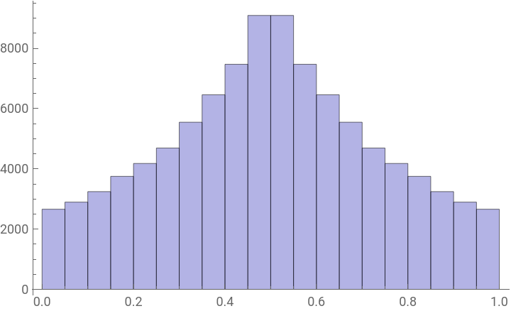
Illustration of the corresponding distributions for N=2 (based on a sample of 50,000 pseudo-randomly generated tuples)
Illustration of the corresponding distributions for N=2 (based on a sample of 50,000 pseudo-randomly generated tuples)
In[]:=
=1;ℓ={};While[≤50000,AppendTo[ℓ,NMcPT[2]];++];Histogram[Flatten[ℓ],ChartStyle->{Opacity[0.3,Darker[Blue]]}]
Out[]=
In[]:=
=1;ℓ={};While[≤50000,AppendTo[ℓ,NMvPT[2]];++];Histogram[Flatten[ℓ],ChartStyle->{Opacity[0.3,Darker[Red]]}]
Out[]=
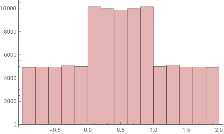
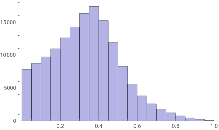
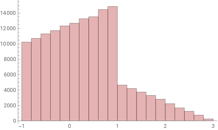
Illustration of the corresponding distributions for N=3 (based on a sample of 50,000 pseudo-randomly generated tuples)
Illustration of the corresponding distributions for N=3 (based on a sample of 50,000 pseudo-randomly generated tuples)
In[]:=
=1;ℓ={};While[≤50000,AppendTo[ℓ,NMcPT[3]];++];Histogram[Flatten[ℓ],ChartStyle->{Opacity[0.3,Darker[Blue]]}]
Out[]=
In[]:=
ListPointPlot3D[ℓ,BoxRatios->{1,1,1},PlotStyleDarker[Blue],ImageSize500]
Out[]=

In[]:=
=1;ℓ={};While[≤50000,AppendTo[ℓ,NMvPT[3]];++];Histogram[Flatten[ℓ],ChartStyle->{Opacity[0.3,Darker[Red]]}]
Out[]=
In[]:=
ListPointPlot3D[ℓ,BoxRatios->{1,1,1},PlotStyleDarker[Red],ImageSize500]
Out[]=

Illustration of the corresponding distributions for N=4 (based on a sample of 50,000 pseudo-randomly generated tuples)
Illustration of the corresponding distributions for N=4 (based on a sample of 50,000 pseudo-randomly generated tuples)
In[]:=
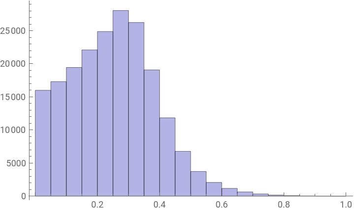
=1;ℓ={};While[≤50000,AppendTo[ℓ,NMcPT[4]];++];Histogram[Flatten[ℓ],ChartStyle->{Opacity[0.3,Darker[Blue]]}]
Out[]=
In[]:=
=1;ℓ={};While[≤50000,AppendTo[ℓ,NMvPT[4]];++];Histogram[Flatten[ℓ],ChartStyle->{Opacity[0.3,Darker[Red]]}]
Out[]=
Illustration of the corresponding distributions for N=5 (based on a sample of 50,000 pseudo-randomly generated tuples)
Illustration of the corresponding distributions for N=5 (based on a sample of 50,000 pseudo-randomly generated tuples)
In[]:=
=1;ℓ={};While[≤50000,AppendTo[ℓ,NMcPT[5]];++];Histogram[Flatten[ℓ],ChartStyle->{Opacity[0.3,Darker[Blue]]}]
Out[]=
Illustration of the corresponding distributions for N=10 (based on a sample of 50,000 pseudo-randomly generated tuples)
Illustration of the corresponding distributions for N=10 (based on a sample of 50,000 pseudo-randomly generated tuples)
Single-qubit state space
Single-qubit state space
Create single-qubit state space with mesh size ϵ
Create single-qubit state space with mesh size ϵ
Generate list of probability vectors
Generate a list with their expectation values
Sanity check #2: Perform sanity check #1 for the new list of probability vectors:
Generate a list with their expectation values
The number of elements in this list is
We can check what percentage of states in the single-qubit state space lie within the Bloch sphere for this particular mesh size, namely
i.e. ≈ 51,6%. [Note: % of states within the Bloch sphere increases with decreasing mesh size ϵ ]
Generate a list with their expectation values
For the mesh size ϵ = 0.005, roughly ≈ 0.0036% [≈ 0.0185%] of states that lie within the Bloch sphere [of all states] are pure states. [Note: % of pure states decreases with decreasing ϵ ]
Generate a list with their expectation values
Sanity check #3:
Let’s check that the entire state space [pv] consists of all states located within the Bloch sphere [qv] plus all states located outside of the Bloch sphere [cv]:
Sanity check #4:
Let’s randomly select 200 states from the Bloch state list and confirm that they lie within the Bloch sphere. The command below will randomly pick 200 elements from the list each time it is executed, i.e. by re-executing the plotting command several times we can check that there is never any point outside of the Block sphere.
Another way to check is to increase the number of randomly selected points. In the limit N to ∞ we should get something that looks like a ball. For one million points, it looks like this:
Of course, we can also illustrate the quantum states as vectors [30 randomly selected states are drawn below].
Lastly, let’s check that our list of pure states is accurate, i.e. all states in this list should lie on the surface of the Bloch sphere.
Note: the plot above can be rotated in all directions, which makes it a bit easier to confirm. Of course, we can also look at the corresponding vectors instead, which may be more easily discernible as ending precisely on the surface of the Bloch sphere.
Sanity check #5:
Let’s randomly select 200 states located outside of the Bloch sphere.
Sanity check #6:
Randomly select states from the entire state space. For ϵ=0.005, ≈48,4% of them should lie outside of the Bloch sphere.
Fig. 1 of arXiv:2312.16281 [quant-ph]
Training data generation and state classification
[1] Generalized Gell-Mann matrix basis
[1] Generalized Gell-Mann matrix basis
[2] Probability tuples and NM breakdown measure γ
[2] Probability tuples and NM breakdown measure γ
Note: The file “ProbabilityTuples.nb” provides a graphical overview of the underlying probability distributions.
Probability tuples for NM-conforming states
Probability tuples for NM-violating states
Function that computes the NM breakdown measure γ for a given vector pvec
[3] Training data generation
[3] Training data generation
Function that generates NM-conforming probability vectors for an arbitrary N-level system.
Function that generates NM-violating probability vectors for an arbitrary N-level system.
Note: For large N it is more efficient to append only the relevant data (e.g. “pv”), but this shall not concern us here.
Note: The counter “ℴ” counts the total number of vectors that have been generated, including those associated with states that do not satisfy the second requirement in Eq. (5.1) of arXiv:2312.16281, which are discarded. As the histogram data generation in [4.1] below illustrates, the efficiency decreases sharpy with increasing N.
[4] Evaluating the NM violation measure
[4] Evaluating the NM violation measure
[4.1] Generating histogram data
[4.1] Generating histogram data
Generate 100,000 NM-violating probability vectors for N=2
Generate 100,000 NM-violating probability vectors for N=2
Generate 100,000 NM-violating probability vectors for N=3
Generate 100,000 NM-violating probability vectors for N=3
Generate 100,000 NM-violating probability vectors for N=4
Generate 100,000 NM-violating probability vectors for N=4
Generate 100,000 NM-violating probability vectors for N=6
Generate 100,000 NM-violating probability vectors for N=6
Generate NM-violating probability vectors for N=7 [evaluation aborted due to long computation time]
Generate NM-violating probability vectors for N=7 [evaluation aborted due to long computation time]
Export lists
Export lists
Export lists of γ values
Export master lists including all probability tuples, density operators, and state vectors
(Note: Large file sizes for large N)
(Note: Large file sizes for large N)
[4.2] Plotting histogram data
[4.2] Plotting histogram data
Import lists of γ values for N ∈ {2,4,6}
Calculate mean γ values
Plot histogram data for N=2
Plot histogram data for N=4
Plot histogram data for N=6
Plot histogram data for N ∈ {2,4,6} in a single histogram
Fig. 2 of arXiv:2312.16281 [quant-ph]
[5] State classification with machine learning
[5] State classification with machine learning
[N=2] (500,000) Single-qubit system
[N=2] (500,000) Single-qubit system
Generate 500,000 NM-conforming probability vectors for N=2
Generate 500,000 NM-violating probability vectors for N=2
Export the generated lists
Store the corresponding probability vectors in a separate list
Assign the value 0 [1] to vectors from the NM-conforming [NM-violating] data set, then join the two lists. The resulting list is the training data for the classifier function.
Train a classifier function based on the training data (i.e. the joined list)
Export the classifier function
Check classification of state from the NM-conforming data set:
Check classification of state from the NM-violating data set:
We can check that this state lies outside of the Bloch sphere to confirm its classification as NM-violating:
If we slightly adjust its components such that it satisfies the Bloch sphere defining inequality, the classifier will correctly identify it as NM-conforming:
[N=3] (500,000)
[N=3] (500,000)
The code for N=3 works analogous to the code for N=2. Note that the input for the classifier function is now a 24-dimensional vector (as opposed to 6-dimensional for N=2).
[N=4] (500,000)
[N=4] (500,000)
The code for N=4 works analogous to the code above. Note that the input for the classifier function is now a 60-dimensional vector.
[N=5] (500,000)
[N=5] (500,000)
The code for N=4 works analogous to the code above. Note that the input for the classifier function is now a 120-dimensional vector.
CITE THIS NOTEBOOK
CITE THIS NOTEBOOK
Probability vector representation of the Schrödinger equation and noninvasive measurability for Leggett-Garg inequalities
by Masahiro Hotta and Sebastian Murk
Wolfram Community, STAFF PICKS, January 17, 2024
https://community.wolfram.com/groups/-/m/t/3104397
by Masahiro Hotta and Sebastian Murk
Wolfram Community, STAFF PICKS, January 17, 2024
https://community.wolfram.com/groups/-/m/t/3104397